Good to see you again. In the previous lesson, you connected a linear score to a probability through odds, log-odds, and the sigmoid function. That transformation is central to logistic regression—but a model also needs a way to determine how changing a parameter changes its loss. Calculus provides that mechanism.
This lesson develops two rules for differentiating a scalar function: the product rule for multiplied functions and the chain rule for nested functions. By the end, you will be able to recognize which rule an expression needs, apply both rules in combination, and trace a simple sigmoid-model loss back to a single model parameter. These are the scalar-calculus foundations for gradients and gradient descent in the next lessons.
First: identify the structure of the function
A derivative measures local sensitivity. If a scalar function has derivative , then for a small input change ,
So is the local multiplier that converts a small change in input into an approximate change in output.
For now, both the input and output are single numbers. The input might be a conventional variable , or it could be one scalar model parameter such as a logistic-regression coefficient .
Before differentiating, inspect the outermost operation in the formula.
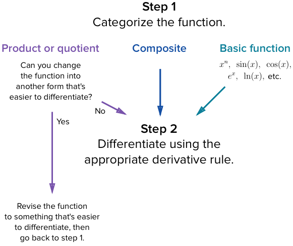
For the scope of this lesson, the important categories are:
| Function | Outermost structure | Main rule |
|---|---|---|
| basic power | power rule | |
| basic trigonometric function | basic derivative rule | |
| one function nested inside another | chain rule | |
| product of two functions | product rule | |
| composite whose inside is a product | chain rule, then product rule |
The most useful preliminary derivative facts are:
Also, derivatives distribute over sums:
The rules in this lesson extend these basic facts to expressions built from multiple pieces.
A small but valuable habit is to simplify only when it genuinely helps. For example,
so differentiating the simplified expression is easier:
But you cannot simplify in a way that avoids reasoning about how both factors change, unless you first expand it accurately.
The product rule: both factors can change
Suppose
is the product of two functions. The product rule is
In words:
Differentiate the first factor and leave the second unchanged, then add the first unchanged factor times the derivative of the second.
A frequent error is to write
This is false. It misses the fact that both factors change as changes.
Why does a sum appear?
Think of as the area of a rectangle with side lengths and . A small input change alters both sides. The resulting area change has:
- a thin strip due to the change in , with approximate area ;
- a thin strip due to the change in , with approximate area ;
- a tiny corner , which becomes negligible compared with in the derivative limit.
That leaves the two main contributions:
Dividing by and taking the limiting rate of change gives the product rule.
Visualizing the chain rule and product rule | Chapter 4, Essence of calculus
Watch “Visualizing the chain rule and product rule” from 3Blue1Brown for geometric intuition behind both rules. The changing-rectangle argument is particularly helpful for seeing why the product rule is a sum rather than a product.
Watch the product-rule visual for the area interpretation of the two terms. Then watch the chain-rule visual, which follows a small input change through a nested function. Focus on what each derivative represents as a local change multiplier, rather than trying to memorize a phrase.
Example: a product involving a power and sine
Let
Define the factors:
Their derivatives are:
Apply the product rule:
Notice that the answer has two terms. The first records how the changing factor affects the product; the second records how the changing sine factor affects it.
A compact mnemonic sometimes used is “left derivative right, plus left right derivative.” The formula is more reliable than the mnemonic:
Keep the undifferentiated factor exactly as it was, evaluated at the original input.
The chain rule: changes pass through nested functions
A composite function has a function inside another function. For example,
has two stages:
- Calculate the inner value:
- Raise that value to the fourth power:
Thus,
The chain rule states:
In standard verbal form:
Differentiate the outside function while keeping the inside unchanged; then multiply by the derivative of the inside.
The derivative of the outside function measures how the final output reacts to a change in the intermediate value . The derivative of the inner function measures how that intermediate value reacts to a change in . Their product gives the final sensitivity to .
A practical template: powers of functions
The most common chain-rule pattern at this stage is:
Then
The final factor is essential. It is the derivative of the inner expression.
Example: a nested power
Return to
Start with the outer operation: “raise something to the fourth power.” Its derivative is
Keep the inner expression in place:
Now multiply by the derivative of the inner expression:
Therefore,
or, after collecting constants,
The incorrect answer
has differentiated the outer layer but ignored the fact that the inner value changes at rate .
A relevant example: sigmoid of a linear score
In the previous lesson, the sigmoid function was
Suppose a one-feature model has score
and probability
This is a composition: the outer function is , and the inner function is .
A useful sigmoid identity is:
Because the inner score has derivative
the chain rule gives:
The multiplier is not optional: it tells us that the score itself changes twice as fast as .
When product and chain rules appear together
Real model expressions often contain both structures. Consider
At the top level, this is a cube of an inner expression, so start with the chain rule:
The derivative left inside is a product, so use the product rule:
Substituting it back gives a clean factored answer:
There is no need to expand this unless a later calculation specifically benefits from expansion. The factored form exposes the computational structure: outer cube, then inner product.
Applying the chain rule and product rule | Advanced derivatives | AP Calculus AB | Khan Academy
Watch “Applying the chain rule and product rule” from Khan Academy for a worked example with exactly this layered structure: an outer power applied to an inner product.
Watch the chain-then-product method. Notice the order: the outer cube produces a chain-rule factor first, and only then does the derivative of the inner product require the product rule. Compare the factored result to the derivation in this lesson.
There can sometimes be more than one valid route. In this example, exponent laws allow
After that rewrite, one could use the product rule first and then the chain rule on . Both routes lead to the same derivative. The best route is generally the one that preserves a clear structure and minimizes algebraic opportunities for error.
A dependable procedure is:
- Locate the outermost operation.
- Apply that rule once.
- Do not alter the inner expression prematurely.
- Differentiate the remaining inner pieces recursively.
- Simplify only after the derivative structure is correct.
From scalar derivatives to a model-loss derivative
The chain rule is the core mechanism by which learning algorithms connect a loss back to the parameters that produced it.
Consider one labeled observation, with:
- feature value ,
- observed binary outcome ,
- scalar weight ,
- fixed intercept .
A logistic model proceeds in three stages:
Here is a squared-error loss for a single observation. It is not the usual preferred loss for logistic regression, but it makes the chain-rule structure especially visible.
When differentiating with respect to , treat , , and as fixed. Trace the calculation from the loss backward:
By applying the chain rule across all three stages,
Thus,
This product has a direct interpretation:
- measures the local error direction and magnitude;
- measures the sigmoid’s local sensitivity;
- measures how strongly changing changes the score.
The full model computation goes forward from to , then , then . The derivative calculation carries sensitivity backward from toward . Later, this same idea will be extended from one parameter to many parameters; that extension is the gradient and, in neural networks, backpropagation.
A numerical sanity check in Python
For a complicated derivative, a central finite-difference approximation can help detect an algebra mistake:
import numpy as np

x = 1.5
y = 1.0
b = -0.3

def sigmoid(z):
    return 1 / (1 + np.exp(-z))

def loss(w):
    p = sigmoid(w * x + b)
    return (y - p) ** 2

def analytic_derivative(w):
    p = sigmoid(w * x + b)
    return 2 * (p - y) * p * (1 - p) * x

w = 0.7
h = 1e-6

finite_difference = (loss(w + h) - loss(w - h)) / (2 * h)

print("Analytic derivative: ", analytic_derivative(w))
print("Finite difference:  ", finite_difference)
The two printed values should be very close. A finite difference is an approximation, not a proof, but it is an effective implementation-level check that your product and chain-rule derivation is plausible.
Key takeaways
The product rule applies when two changing functions are multiplied:
The chain rule applies when one function is nested inside another:
For powers of an inner function:
The main procedural skill is not memorizing a large list of rules. It is accurately reading an expression’s structure: identify its outer operation, differentiate one layer, and continue inward until every changing component has been accounted for.
Next, you will extend this scalar reasoning to losses with several parameters by computing gradients from partial derivatives.