Understanding Dynamic Emotional Responses

The Psychology of Changing Responses

Before we dive into the statistical plots, let's establish a conceptual foundation for why effects change over time. Two key psychological processes, habituation and sensitization, often operate in tandem to shape our responses to repeated stimuli.

As the video explains, the observed behavior is a summation of the habituation and sensitization processes. In your context:

• Habituation could manifest as the husband's jealousy diminishing over repeated encounters, even if each encounter is similar. The stimulus (e.g., wife's date) becomes less potent over time.
• Sensitization could occur if repeated encounters, instead of dulling the response, actually heighten emotional sensitivity. For instance, the wife's guilt might build cumulatively with each date, or the husband's jealousy could be amplified by ruminative thoughts between encounters.

The key takeaway is that the change in an emotional response is not random; it's often the product of underlying, competing psychological mechanisms. Our statistical models are tools to reveal the net outcome of these processes.

From Parametric Curves to Dynamic Patterns

In the previous lesson, we touched on using polynomial terms (e.g., an interaction between an activity and time-squared) to model non-linear changes. This is a simple, parametric way to look for habituation or sensitization.

A significant negative quadratic effect, for example, would describe a curve that flattens out over time, suggesting diminishing returns or habituation. This is a common pattern in skill acquisition and therapeutic processes.

While useful, this parametric approach forces the change to fit a specific shape (e.g., a parabola). For a more exploratory, data-driven approach, we turn to the non-parametric methods we introduced last time, which allow us to discover the shape of change.

Interpreting Time-Varying Effect Model (TVEM) Plots

The primary output of a TVEM is not a single number, but a set of plots showing how the intercept ${\beta }_0(t)$ and slope coefficients ${\beta }_k(t)$ change as a function of time.

Let's ground this in the foundational TVEM paper.

The paper uses P-splines to estimate these functions. As you know from your statistical background, this is a method of flexible regression that approximates a smooth function using a series of basis functions, with a penalty to prevent overfitting. The result is a data-driven estimate of the coefficient's trajectory over time.

Let's look at the hypothetical coefficient functions from Figure 2 of the paper.

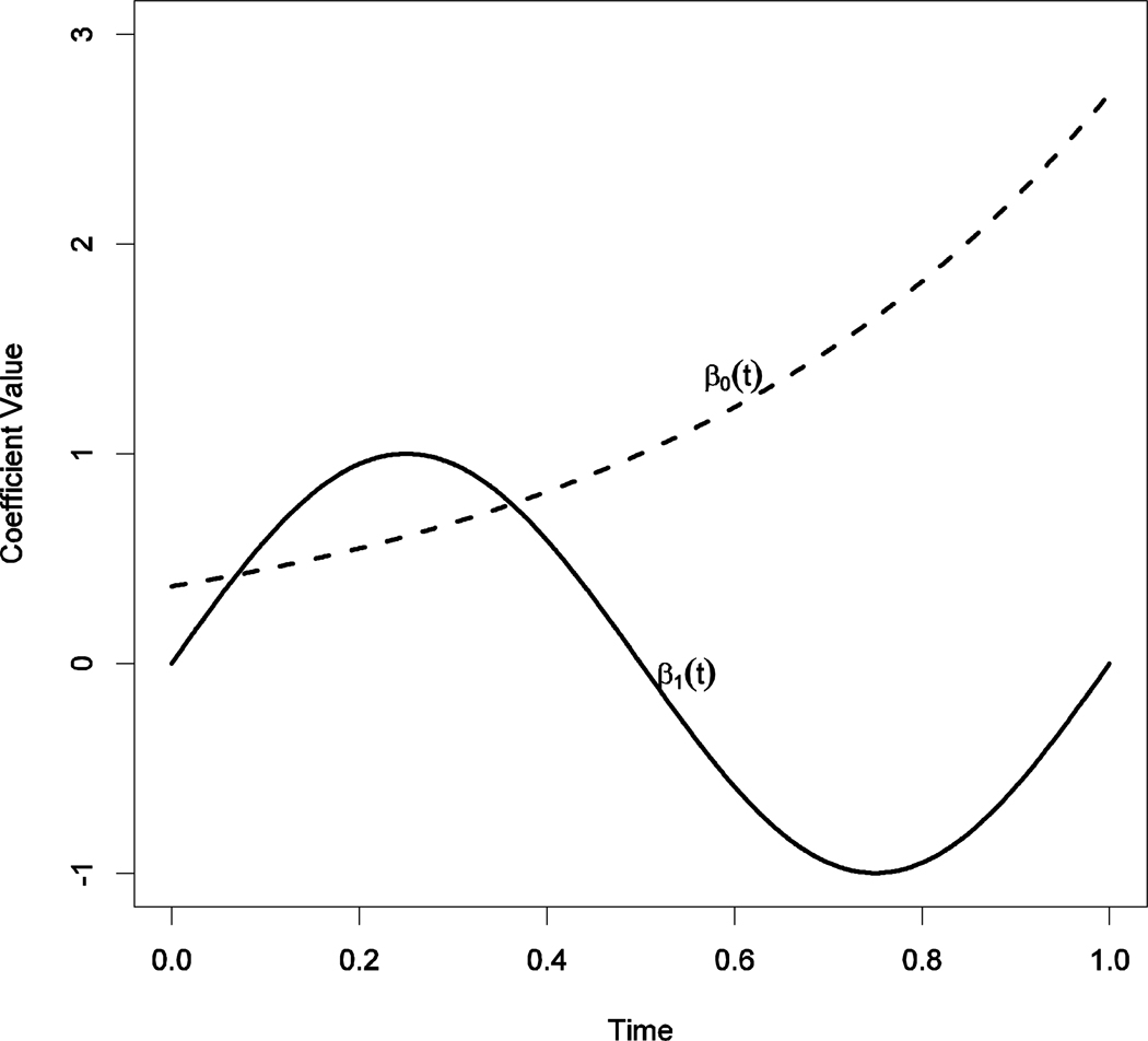
Here's how to interpret the solid line, ${\beta }_1(t)$, which represents the changing effect of a predictor X on an outcome Y:

• At Time = 0.0, the slope is 0. X has no effect on Y.
• At Time = 0.25, the slope reaches its peak at 1.0. This is where X has its strongest positive effect on Y.
• At Time = 0.5, the slope is 0 again. The effect has vanished.
• At Time = 0.75, the slope reaches its minimum at -1.0. Here, X has its strongest negative effect on Y.
• At Time = 1.0, the slope returns to 0.

This is a cyclical effect. In your research, this could model a "honeymoon and hangover" effect. For example, the effect of a communication intervention (the predictor) on relationship satisfaction (the outcome) might be initially positive, then fade, and then become negative as the novelty wears off and the effort feels like a chore, before eventually leveling off.

Now let's examine the plots from the paper's simulated example, which show the model recovering known patterns.

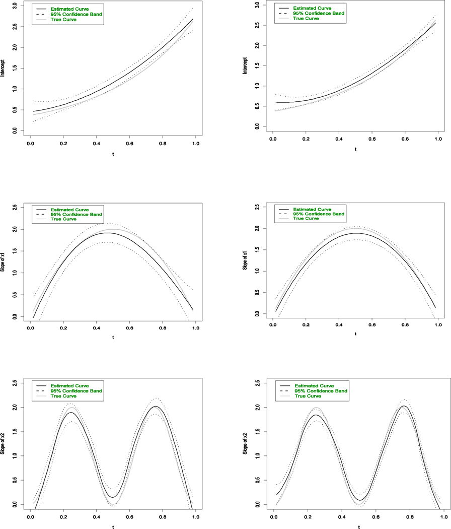
• Middle Row (Slope of x1): This shows a clear quadratic pattern. The effect of x1 on the outcome is initially zero, increases to a peak around t=0.5, and then decreases back to zero. This is a pattern of an effect emerging and then habituating. If this were the effect of "wife's disclosure" on "husband's jealousy," it would suggest that disclosure is most impactful mid-way through the process, but its effect diminishes as the husband becomes accustomed to it.
• Bottom Row (Slope of x2): This shows a clear sinusoidal or cyclical pattern, similar to the hypothetical one we just discussed. The effect of x2 oscillates between positive and less positive over time. This could represent natural ebbs and flows in emotional influence, perhaps tied to external weekly schedules or internal hormonal cycles.

Case Study: Interpreting Dyadic Dynamics with TV-VAR

The Time-Varying Vector Autoregressive (TV-VAR) model extends these ideas to a multivariate system, making it perfect for dyadic and triadic data. Instead of just one $\beta (t)$, we can now estimate time-varying autoregressive effects (emotional inertia) and time-varying cross-lagged effects (emotional influence between partners).

Let's break down the interpretation of the results for the male's positive affect (PA) in that paper (Figure 10):

• Intercept (${\beta }_{10,t}$): This function shows the male's expected PA on a given day when his and his partner's PA on the previous day were zero. It shows a slight downward trend, indicating his baseline mood may have been slowly decreasing over the 91 days.
• Autoregressive Effect / Inertia (${\beta }_{11,t}$): This is the effect of the male's own PA on his PA the next day. The authors found this function to be essentially flat and positive. This means he had a stable, moderate level of emotional inertia; his positive mood tended to carry over from one day to the next, and this tendency did not change over the study period.
• Cross-Lagged Effect (${\beta }_{12,t}$): This is the most interesting part. It represents the effect of the female's PA on the male's PA the next day. The plot shows that for the first ~45 days, this effect was zero (the confidence interval includes zero). Her mood had no discernible effect on his. However, around day 45, the effect becomes negative and significant. This is a pattern of emerging influence or sensitization to the partner. After day 45, when her PA was high, his tended to be lower the next day, and vice-versa. A static model would have averaged this out to a small, possibly non-significant effect, completely missing the crucial change in their dynamic.

This is a powerful demonstration of what TVEM/TV-VAR can reveal. For your research, you could generate similar plots to answer questions like:

• Does the effect of the bull's communication style on the wife's guilt habituate over time? (i.e., does the $\beta (t)$ curve for this effect trend towards zero?).
• Does the husband become sensitized to details of the encounters, meaning the effect of disclosure on his jealousy grows stronger over time? (i.e., does the $\beta (t)$ curve trend away from zero?).
• Is there a cyclical pattern to the influence, where the wife's guilt after a date has a strong effect on the husband's jealousy one week, but a weak effect the next?

Conclusion

In this lesson, we have moved from specifying models to interpreting their rich, dynamic output. You now have a framework for translating the shapes of coefficient functions into substantive conclusions about the evolution of emotional responses.

Key Takeaways:

• Time-varying effect patterns like habituation (effect weakens), sensitization (effect strengthens), and cyclical effects (effect oscillates) can be visualized and interpreted using the coefficient function plots from TVEM and TV-VAR models.
• A coefficient function $\beta (t)$ trending towards zero indicates habituation.
• A coefficient function $\beta (t)$ trending away from zero (either more positive or more negative) indicates sensitization.
• An oscillating coefficient function $\beta (t)$ indicates a cyclical or periodic effect.
• Interpreting these plots allows you to tell a much more nuanced story about how relationships evolve, revealing dynamics that static models would average out and obscure.

This ability to analyze how effects change over time is not just an analytical curiosity; it is a critical prerequisite for effective intervention. This brings us to the next module, Designing Experiments for Triadic Interventions. If you know from a TVEM analysis that an intervention's positive effect habituates after ten sessions, you can design your experiment to include a "booster" session at week 11. If you know an effect is cyclical, you can design your measurements to capture both the peaks and the troughs. Your understanding of dynamic effects now enables you to design smarter, more effective experiments.