Visualizing Time Series Data

1. The Foundational Line Plot: Your First Look at the Data

The first and most important visualization for any time series is a simple line plot of the value against time. This single chart provides a high-level overview and can immediately reveal dominant characteristics like long-term trends, repeating seasonal patterns, and obvious outliers.

Now, let's see this in practice. While Matplotlib is excellent for static plots, modern interactive libraries like Plotly can make exploration much more dynamic. The following video uses Plotly Express, a high-level wrapper that makes creating beautiful, interactive plots very straightforward.

As you saw, a simple call to px.line() after grouping the data gives you a powerful, interactive view. This is your starting point for forming hypotheses about the data. Do you see a trend? Is there a repeating pattern? Are there any strange spikes or drops?

2. Visualizing Specific Patterns and Distributions

Once the overall line plot gives you some clues, the next step is to zoom in and confirm those patterns. We often want to investigate seasonality at different frequencies (e.g., weekly, monthly, yearly).

Bar Charts for Cyclical Timeframes

If you suspect a weekly pattern (e.g., sales are higher on weekends), you can't easily see that in a plot spanning several years. A better approach is to group the data by the day of the week and plot the average or total values using a bar chart.

The next clip from Jeff Heaton's video demonstrates this perfectly.

Box Plots for Deeper Distributional Insights

While a bar chart shows an aggregate value (like the mean or sum), a box plot gives you a much richer view of the distribution of values for each period. It shows the median, interquartile range (IQR), and potential outliers, all in one compact visualization. This is excellent for comparing distributions and spotting anomalies.

The following video explores a dataset of energy consumption and uses box plots to analyze monthly patterns.

3. Smoothing to Clarify Trends

Time series data is often "noisy," meaning it has random, short-term fluctuations. This noise can make it difficult to see the underlying trend. A common technique to address this is to calculate a moving average (also called a rolling average). This smooths out the noise by averaging data points over a specified time window.

Your pandas skills are directly applicable here, using the .rolling() method.

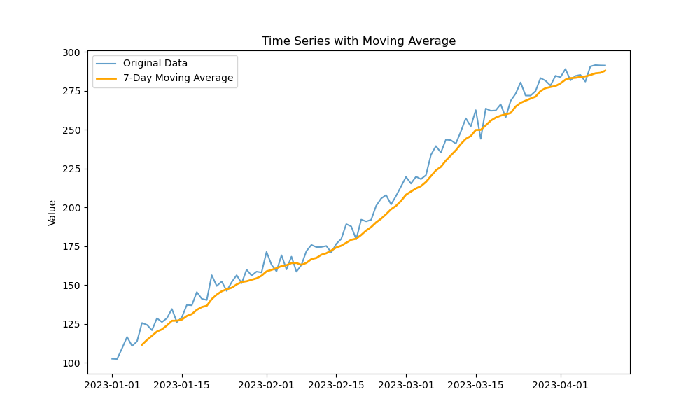
Here is a typical code snippet to generate such a plot, assuming your data is in a pandas Series ts_data:

import matplotlib.pyplot as plt

# Calculate the 7-day moving average
moving_avg = ts_data.rolling(window=7).mean()

# Plot the original data and the moving average
plt.figure(figsize=(12, 6))
plt.plot(ts_data, label='Original Data')
plt.plot(moving_avg, label='7-Day Moving Average', color='orange')
plt.title('Time Series with Moving Average')
plt.legend()
plt.show()

4. Visualizing Data Quality and Anomalies

Visualization isn't just for finding modeling patterns; it's also a powerful diagnostic tool for identifying data quality issues.

A particularly useful technique for multivariate datasets (like sensor data) is to visualize when data points are missing. Spikes, dips, or flat lines in the main time series plot can indicate anomalies, but plotting the absence of data can be just as revealing.

5. Visualizing Multiple Time Series

When working with multivariate data, you need ways to understand the relationships between the different series.

Correlation Heatmaps

A correlation matrix heatmap is a fantastic tool for getting a quick overview of the linear relationships between all pairs of time series in your dataset. It helps you answer questions like: "Do series A and B tend to move together?" or "Do they move in opposite directions?"

Overlaying and Faceting Plots

After a heatmap identifies interesting pairs, you can plot them together on a line chart to visually confirm their relationship.

For comparing more than a handful of series, overlaying them on a single plot can become a "spaghetti plot" — tangled and unreadable. A cleaner approach is to use "small multiples" or faceted charts, where each time series gets its own small graph, but they all share the same time axis. This makes side-by-side comparison much easier.

Conclusion

You've now learned the fundamental techniques for visualizing time series data. This is an exploratory and iterative process. A good visualization can confirm a hypothesis, reveal an unexpected pattern, or flag a data quality issue that needs to be addressed before modeling.

Key Takeaways:

• Start with a Line Plot: It's your primary tool for seeing the overall trend, seasonality, and obvious anomalies.
• Use Bar and Box Plots for Seasonality: Aggregate your data by a time period (day of week, month) to create bar charts (for totals/means) or box plots (for distributions) to confirm seasonal patterns.
• Smooth with Moving Averages: Use rolling().mean() to smooth out noise and clarify the underlying trend.
• Visualize Data Quality: Plotting missing values or other data quality metrics over time is a critical diagnostic step.
• Analyze Multiple Series: Use correlation heatmaps for a high-level overview and faceted plots for clear side-by-side comparisons.

In our next lesson, we will move from visual exploration to statistical analysis. We will learn how to formally decompose a time series into its trend, seasonal, and residual components, putting a mathematical structure on the patterns we've learned to identify by eye today.