Introduction
Welcome to our next lesson. In our previous discussions on the Weak and Strong Laws of Large Numbers, we established that the sample mean converges to the true mean as the sample size grows. This tells us where the average is heading. However, it doesn't describe the nature of the fluctuations around for a large but finite . What is the distribution of the error, ? And at what rate does this error shrink?
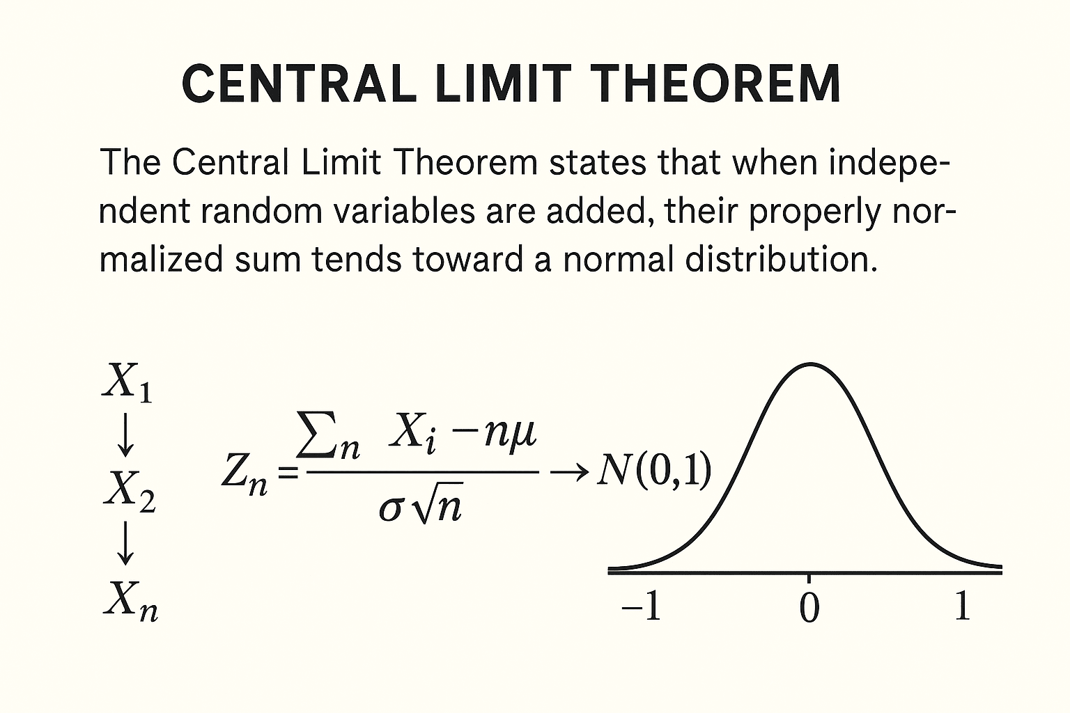
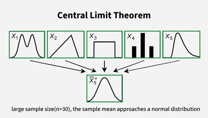
Today, we address these questions with the Central Limit Theorem (CLT), arguably one of the most remarkable and foundational results in all of probability and statistics. The CLT states that the distribution of the properly normalized sample mean of i.i.d. random variables converges to a standard normal distribution, regardless of the original distribution of the variables, as long as they have a finite variance. This universal emergence of the Gaussian bell curve explains its prevalence in nature and its central role in statistical inference.
In this lesson, you will learn to state the formal Central Limit Theorem for i.i.d. variables, understand the mechanics of its proof, and apply it to approximate probabilities that are otherwise difficult to calculate.
Stating the Central Limit Theorem
The most common version of the CLT, often called the Lindeberg-Lévy CLT, applies to independent and identically distributed (i.i.d.) random variables.
Theorem (Central Limit Theorem):
Let be a sequence of i.i.d. random variables with a finite mean and a finite, positive variance .
Let be the sample mean. Then the standardized sample mean,
converges in distribution to a standard normal random variable as .
This is written as:
Formally, this means the cumulative distribution function (CDF) of converges to the CDF of the standard normal distribution, :
Key Insights from the Theorem
-
Universality: The striking feature is that the limiting distribution is always normal. The original distribution of the can be discrete (like Bernoulli or Poisson) or continuous (like Uniform or Exponential), symmetric or skewed. As long as the variance is finite, their sum, when appropriately scaled, will be approximately normal.
-
Rate of Convergence: The factor is crucial. The Laws of Large Numbers tell us that goes to zero. The CLT gives a more precise statement: the typical magnitude of the error is on the order of . Multiplying by "zooms in" on the fluctuations at the correct scale to reveal a stable, non-degenerate distribution.
-
Convergence in Distribution: The CLT guarantees convergence of the CDFs, which is a weaker mode of convergence than the almost sure convergence of the SLLN. The random variable itself does not converge to a single value, but its probabilistic character becomes indistinguishable from a standard normal.
The following video provides an excellent introduction, distinguishing the CLT from the LLN and highlighting its significance.
Lecture 29: Law of Large Numbers and Central Limit Theorem | Statistics 110
In this first segment from Harvard's Statistics 110 course, Professor Joe Blitzstein introduces the Central Limit Theorem, contrasting it with the Law of Large Numbers and explaining its role in describing the distribution and convergence rate of the sample mean.
Please watch from the beginning to 02:07 and from 15:27 to 22:15. Focus on: The setup with i.i.d. random variables. How the CLT addresses the distribution and rate of convergence, which the LLN does not. The formal statement of the theorem and the meaning of convergence in distribution. The amazing generality of the result: the starting distribution doesn't matter, only that it has a finite variance.
The Proof of the Central Limit Theorem
The standard proof of the Lindeberg-Lévy CLT is a beautiful application of transform methods. The strategy hinges on a fundamental result called Lévy's Continuity Theorem, which states that convergence in distribution of a sequence of random variables is equivalent to the pointwise convergence of their characteristic functions (or moment generating functions, if they exist in a neighborhood of zero).
The proof proceeds as follows:
- Goal: Show that the MGF of the standardized mean, , converges to , which is the MGF of a random variable.
- Simplify: Without loss of generality, assume the original variables are already standardized, i.e., and . If not, we can just define and proceed. In this case, .
- Use MGF Properties: The MGF of a sum of independent variables is the product of their MGFs. The MGF of a scaled variable is . Combining these gives .
- Taylor Expansion: Expand around : .
- Use Moments: By definition, , , and . So, .
- Substitute and Take the Limit: Substitute into the expansion and take the -th power. This results in an expression of the form . As , this converges to by the definition of the exponential function, .
The following two videos walk through this proof with excellent clarity. They use slightly different techniques for the final limit (L'Hôpital's Rule vs. Taylor series), offering two robust perspectives on the same core logic.
Lecture 29: Law of Large Numbers and Central Limit Theorem | Statistics 110
This segment from the Harvard lecture provides a full proof of the CLT, assuming the MGF exists. The proof cleverly uses L'Hôpital's rule twice to handle the indeterminate form that arises.
Please watch from 24:33 to 37:40. Follow the steps of finding the MGF of the standardized sum and then taking the limit. Pay attention to how the problem is simplified by assuming \mu=0, \sigma=1 and how the log-transform helps in applying L'Hôpital's rule.
Proof of the Central Limit Theorem
This video by Steve Brunton offers another clear, step-by-step derivation of the CLT proof, also using MGFs. This version emphasizes the role of the Taylor series expansion of the MGF.
Watch the video from 00:52 to 20:34. This provides a complete walk-through of the proof strategy. Notice how the coefficients of the Taylor expansion of the MGF correspond directly to the moments of the distribution, which is why this method works so elegantly.
For completeness, it's worth noting that the most general proofs use characteristic functions (CFs), which are related to the Fourier transform and exist for all probability distributions, unlike MGFs. The logic is identical. The document below provides a concise proof using CFs.
[PDF] CHAPTER 4. LIMIT THEOREMS IN STATISTICS
This document from a course at UC Berkeley provides a formal statement of the Lindeberg-Levy CLT and a concise proof using characteristic functions.
Read the section '4.4. CENTRAL LIMIT THEOREMS', focusing on Theorem 4.10 and its proof. You will see that the structure is the same as the MGF proof: expand the CF, use the moments, and take the limit.
Applying the Central Limit Theorem
The primary application of the CLT is to approximate the distribution of a sample mean or a sum. For a large , we can treat as if it were drawn from a normal distribution:
Similarly, the sum is approximately normal:
Example: Normal Approximation to the Binomial
A classic application is approximating binomial probabilities. A random variable represents the number of successes in trials and can be viewed as the sum of i.i.d. random variables.
For a Bernoulli variable, and .
Therefore, for the sum , we have and .
By the CLT, for large , is approximately normally distributed with this mean and variance. This is invaluable because calculating exact binomial probabilities, , can be computationally intensive for large .
Continuity Correction: When approximating a discrete distribution (like the Binomial) with a continuous one (like the Normal), accuracy is improved by using a continuity correction. The probability mass at a single integer value in the discrete distribution is represented by the area over the interval in the continuous approximation.
- To approximate , we compute .
- To approximate , we compute .
- To approximate , we compute .
The following video demonstrates this application, including the continuity correction.
Lecture 29: Law of Large Numbers and Central Limit Theorem | Statistics 110
The final part of the Harvard lecture illustrates how to apply the CLT to approximate binomial probabilities, explaining the rationale behind the continuity correction.
Watch from 37:40 to 49:05. Pay close attention to: The conditions under which the normal approximation to the binomial is valid (in contrast to the Poisson approximation). The step-by-step process of standardizing the binomial variable. The clear explanation of why the continuity correction is necessary and how to apply it.
Conclusion
The Central Limit Theorem is a cornerstone of statistical theory, providing the justification for why the normal distribution appears so frequently in applied problems.
Key Takeaways:
- The Central Limit Theorem states that the distribution of the standardized sample mean of i.i.d. variables with finite variance converges to a standard normal distribution.
- This result is universal, holding regardless of the shape of the parent distribution.
- The correct scaling factor is , which describes the rate at which the sample mean approaches the true mean.
- The standard proof uses moment generating functions or characteristic functions, relying on Taylor expansions and the properties of limits.
- A key application is the normal approximation of other distributions, like the Binomial, which is made more accurate by using a continuity correction.
Preview of the Next Lesson:
The CLT provides the asymptotic distribution for the sample mean . But what if we are interested in a parameter that is a function of the mean, such as or ? How do we find the distribution of these transformed estimators? In our next lesson, we will introduce the delta method, a powerful tool that combines the CLT with a Taylor series approximation to derive the asymptotic distributions of functions of random variables.