BST Time Complexity: Balanced vs. Unbalanced

The Central Role of Tree Height ($h$)

Let's start by establishing a fundamental rule. The three most common operations on a BST are searching for a value, inserting a new value, and deleting a value. All three begin the same way: by traversing from the root downwards to find the target node or the correct position for a new node.

This downward path is the dominant part of the work. The number of comparisons needed is directly proportional to the length of this path, which, in the worst case, is the height of the tree, $h$. Therefore, the time complexity for all these operations can be summarized as $O(h)$.

To see this pattern clearly, let's examine a resource that breaks down the complexity for each operation.

Now that we've established that the complexity is $O(h)$, the crucial question is: what can the value of $h$ be in relation to $n$, the number of nodes?

The Two Extremes: Balanced vs. Unbalanced

The height of a BST can vary dramatically depending on the sequence of insertions. This leads to two main scenarios: the worst case (an unbalanced tree) and the best case (a balanced tree).

The Unbalanced Tree: Worst-Case Complexity of $O(n)$

Imagine we build a BST by inserting numbers that are already in sorted order, like [10, 20, 30, 40, 50].

• We insert 10. It becomes the root.
• We insert 20. It's greater than 10, so it goes to the right.
• We insert 30. It's greater than 10 and 20, so it goes to the right of 20.
• ...and so on.

The resulting tree is "skewed" or "degenerate"—it's effectively a linked list.

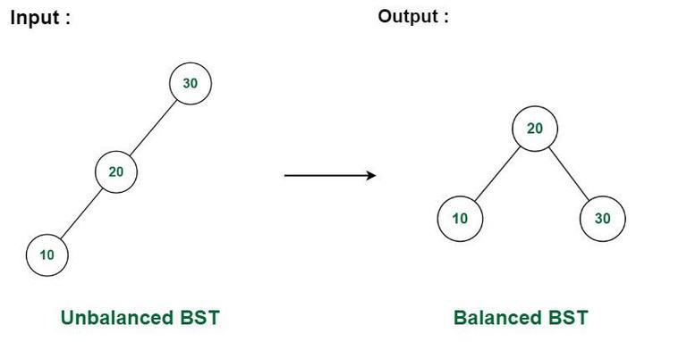
In this worst-case scenario, a tree with $n$ nodes has a height of $h\approx n$. If we need to search for the last element, we must traverse all $n$ nodes. This makes our BST operations no better than a linear search through a list.

Worst-Case Complexity: $O(n)$

The Balanced Tree: Best-Case Complexity of $O(\log n)$

Now, what if the tree is "balanced" or "bushy," with nodes distributed as evenly as possible between the left and right subtrees? In this case, the tree's height is minimized.

This is where your math background with logarithms comes into play. In a perfectly balanced binary tree, each level down roughly doubles the number of nodes. To find the height $h$ for a tree with $n$ nodes, we're essentially asking: how many times do we have to double 1 to get to $n$? This is the definition of a base-2 logarithm.

So, for a balanced tree with $n$ nodes, the height is $h\approx {\log }_{2}n$. Since each BST operation takes $O(h)$ time, the complexity becomes $O(\log n)$.

The following resource provides an excellent, multi-faceted explanation for this logarithmic relationship.

This logarithmic performance is incredibly efficient. To put it in perspective, for a balanced tree with a million nodes, a search would take about 20 steps (${\log }_{2}1,000,000\approx 20$), whereas in an unbalanced tree, it could take a million steps.

Applying Best- and Worst-Case Analysis

We now have two extremes for our BST's performance: $O(\log n)$ and $O(n)$. Let's formalize this using the concepts of best- and worst-case analysis.

A key insight is that the "worst case" for a search operation is usually finding a leaf node (or discovering a value isn't there), because that requires the longest path. However, the time taken for that worst-case search depends on the tree's structure.

• A balanced tree gives us the best-case time complexity for our operations: $O(\log n)$.
• An unbalanced tree gives us the worst-case time complexity: $O(n)$.

The following videos will help solidify this distinction.

Hands-On: A Python Experiment

Let's see this theory in action. We'll write a small script to measure the number of steps it takes to find an element in a balanced-like tree versus a perfectly unbalanced tree.

We'll need to modify our search method slightly to count the steps.

Copy the following code into a file named bst_complexity_test.py and run it.

import random

class BinarySearchTreeNode:
    def __init__(self, data):
        self.data = data
        self.left = None
        self.right = None

    def add_child(self, data):
        if data == self.data:
            return
        if data < self.data:
            if self.left:
                self.left.add_child(data)
            else:
                self.left = BinarySearchTreeNode(data)
        else:
            if self.right:
                self.right.add_child(data)
            else:
                self.right = BinarySearchTreeNode(data)

    def search_with_count(self, val):
        """Searches for a value and returns a tuple: (found_boolean, steps_taken)."""
        steps = 1 # Count the current node as one step
        current = self
        while current:
            if val == current.data:
                return (True, steps)
            elif val < current.data:
                current = current.left
            else:
                current = current.right
            
            if current: # Only increment steps if we are moving to another node
                steps += 1
        
        return (False, steps)

def build_tree(elements):
    if not elements:
        return None
    root = BinarySearchTreeNode(elements[0])
    for i in range(1, len(elements)):
        root.add_child(elements[i])
    return root




# --- Main part of the script ---
if __name__ == '__main__':



    # Create a list of numbers from 0 to 999
    numbers = list(range(1000))
    



    # --- Case 1: Unbalanced Tree ---
    # Build a tree from sorted data. This will create a skewed tree.
    unbalanced_tree = build_tree(numbers)



    # Search for the last element, which is at the deepest point.
    found, steps = unbalanced_tree.search_with_count(999)
    print(f"Unbalanced Tree (sorted insertion):")
    print(f"Searching for 999 took {steps} steps.\n")




    # --- Case 2: More Balanced Tree ---
    # Shuffle the numbers to get a random insertion order.
    random.shuffle(numbers)



    # This is likely to create a more balanced tree.
    balanced_tree = build_tree(numbers)



    # Search for the same element.
    found, steps = balanced_tree.search_with_count(999)
    print(f"More Balanced Tree (random insertion):")
    print(f"Searching for 999 took {steps} steps.")
    print(f"(For reference, log2(1000) is approximately {1000:0.2f})")

When you run the script, you should see a dramatic difference. The search in the unbalanced tree will take around 1000 steps, while the search in the randomized (and thus more balanced) tree will take a number of steps much closer to ${\log }_{2}1000\approx 10$.

Conclusion

Great job today! You've tackled one of the most important concepts in algorithm analysis: understanding how a data structure's performance can vary between best and worst-case scenarios.

Key Takeaways:

• The time complexity of BST search, insertion, and deletion is fundamentally tied to the tree's height, $h$, making them all $O(h)$ operations.
• An unbalanced (skewed) tree represents the worst case, where $h\approx n$. This results in a linear time complexity of $O(n)$.
• A balanced tree represents the best case, where $h\approx \log n$. This results in a highly efficient logarithmic time complexity of $O(\log n)$.
• The shape of the tree, and therefore its performance, is determined by the order in which elements are inserted. Random insertion tends to produce better-balanced trees than sorted insertion.

Preview of the Next Lesson:

Now that you have a firm grasp of BST structure, traversals, and complexity, it's time to solve a common practice problem. In the next lesson, you will solve a practice problem involving a BST, such as finding the minimum value. As you think about it, consider what the time complexity of finding the minimum value would be in both a balanced and an unbalanced tree.