Hash Table Time Complexity

The Two Faces of Hash Table Performance

As you've learned, Big O notation helps us describe how an algorithm's runtime scales with input size. A great algorithm is one that remains fast even as the data grows.

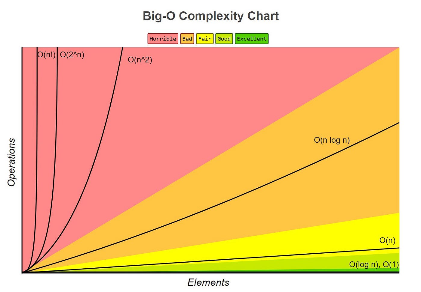
The remarkable thing about a hash table is that its performance can either be O(1) or O(n), depending on how well the keys are distributed. Let's explore these two scenarios.

The Average Case: O(1) Constant Time

In a typical, well-functioning hash table, operations are considered to have an average time complexity of O(1). This means that, on average, the time it takes to search for, insert, or delete an item is constant, regardless of how many items are in the table. This is the "magic" of hash tables.

How is this possible, especially with collisions? It relies on three key factors working together.

As you just read, the three pillars of O(1) performance are:

1. A Good Hash Function: It distributes keys uniformly across the array. This prevents keys from clustering in a few buckets and ensures the chains remain short.
2. Efficient Collision Resolution: Separate chaining provides a simple way to handle the few collisions that do occur.
3. A Low Load Factor: The load factor is the ratio of stored elements to the number of buckets (n/m). By keeping this ratio low (e.g., below 0.75), we ensure there's plenty of space, making long chains statistically unlikely. If the load factor gets too high, the hash table is resized (a process called rehashing) to maintain performance.

When these conditions are met, the average length of a chain is a small, constant number. A search operation then consists of:

• Computing the hash: O(1)
• Accessing the bucket (array index): O(1)
• Searching a tiny list (e.g., 1 or 2 items): O(1)

The total time is constant. The same logic applies to insert and delete.

The Worst Case: O(n) Linear Time

Now, let's consider the worst-case scenario. What if our hash function is terrible? Imagine a function that, for some reason, hashes every single key to the same index, say index 2.

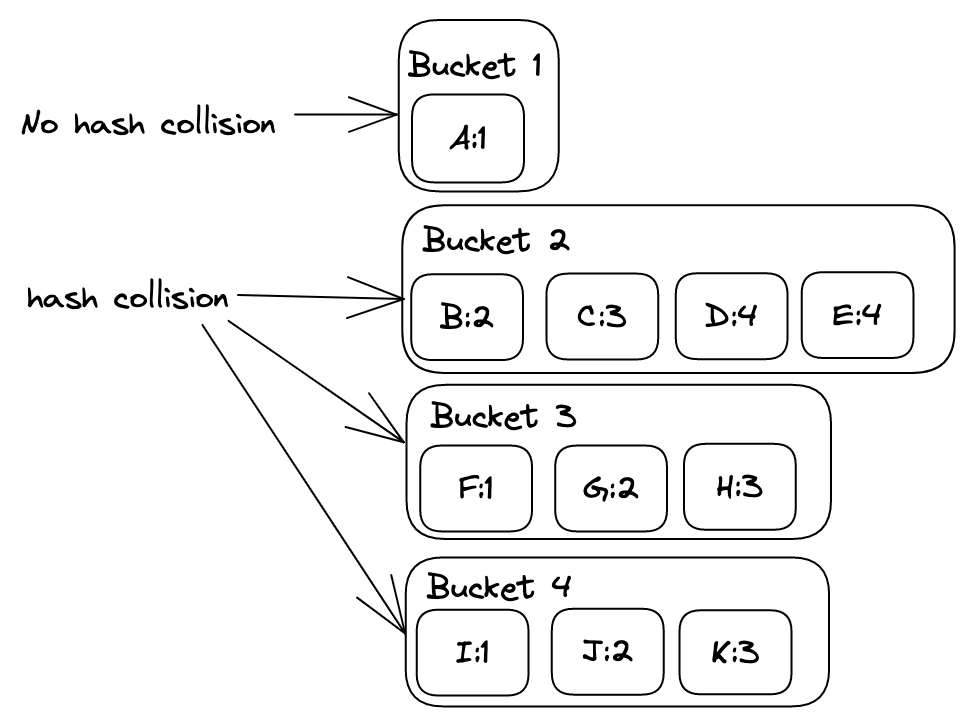
If all n items we insert collide and end up in the same bucket, our hash table no longer provides a benefit. That one bucket becomes a single linked list containing all n items.

In this situation:

• Search: To find an item, we compute the hash (O(1)), jump to the correct bucket (O(1)), and then perform a linear search through a linked list of n items. The dominant cost is the linear search, making the overall complexity O(n).
• Insert/Delete: Similarly, these operations would first require searching the list, taking O(n) time.

This worst-case scenario effectively degrades the hash table into a simple linked list, losing all its performance advantages.

Let's watch two short video clips that summarize the best, average, and worst cases clearly.

To complete your reading, let's look at the "Worst Case" part of the Youcademy article.

Why Average Case is What Matters

At this point, you might be worried about the O(n) worst case. The good news is that in any practical, well-implemented hash table (like Python's dictionary), the worst case is extremely rare.

Hash functions used in modern programming languages are carefully designed to provide uniform distribution. Furthermore, automatic resizing and rehashing ensure the load factor stays low. Because of this careful engineering, we can confidently rely on the O(1) average time complexity for our analysis and when choosing data structures.

This is a key point for technical interviews: you should be able to explain both the average and worst-case complexities and, crucially, articulate why the average case is the one we usually encounter in practice.

Conclusion

In this lesson, we dissected the performance of hash tables, a cornerstone topic for understanding data structures.

Key Takeaways:

• The average-case time complexity for hash table insertion, deletion, and search is O(1). This is achieved through a combination of a good hash function, an efficient collision resolution strategy (like chaining), and maintaining a low load factor.
• The worst-case time complexity is O(n). This occurs when a poor hash function causes all (or most) keys to collide into a single bucket, turning the hash table into an inefficient linked list.
• In practice, due to clever design and optimizations in standard library implementations, the O(1) average-case performance is what makes hash tables so fast and useful.

Preview of the Next Lesson:

Now that you have a solid theoretical understanding of how hash tables work and why they are so efficient, it's time to put them into practice. In the next lesson, we will learn how to use Python's built-in dictionary, which is a highly optimized hash table implementation, to solve problems that require fast lookups.