Instantaneous Velocity: Limits and Geometric Interpretation

Hello! Welcome to the third lesson in our exploration of kinematics.

In our previous session, we delved into the calculus of vectors in moving coordinate systems. We frequently used the notation $v = \frac{d r}{d t}$ to represent velocity as the time derivative of the position vector. However, we treated this relationship as a given. Your goal for a "hyper deep" understanding demands that we build this concept from the ground up.

Today, we will address the learning outcome: Derive instantaneous velocity from average velocity using limits and interpret its geometric meaning on position-time graphs. We will rigorously define what the derivative $\frac{d r}{d t}$ truly means in a physical context. This lesson forms a crucial bridge between the intuitive idea of "speed" and the powerful mathematical framework of calculus that underpins all of physics.

1. The Inadequacy of Average Velocity

Let's begin with a concept you're likely familiar with: average velocity. For one-dimensional motion, if an object is at position $x_{1}$ at time $t_{1}$ and later at position $x_{2}$ at time $t_{2}$ , its average velocity is the displacement divided by the time interval:

v ˉ = \frac{x _{2} - x _{1}}{t _{2} - t _{1}} = \frac{Δ x}{Δ t}

While simple, average velocity has a significant limitation. If you travel 120 km from one city to another in 2 hours, your average velocity is 60 km/h. But this single number tells you nothing about your velocity at any specific moment during the trip. You might have been stuck in traffic at 0 km/h for a while and later traveled at 100 km/h on a highway.

To describe the motion precisely at a single instant, we need the concept of instantaneous velocity.

2. The Limiting Process: From Average to Instantaneous

The path to defining instantaneous velocity lies in a thought experiment. Imagine you want to know your velocity exactly at time $t$ . You could measure your average velocity over a very short time interval, say from $t$ to $t + Δ t$ .

The average velocity over this interval is:

v ˉ = \frac{x ( t + Δ t ) - x ( t )}{Δ t}

If you make the time interval $Δ t$ smaller and smaller, the average velocity you calculate becomes a better and better approximation of your velocity right at the instant $t$ . The instantaneous velocity is what this average velocity approaches as the time interval $Δ t$ shrinks to zero.

This is precisely the mathematical concept of a limit. We formally define instantaneous velocity, $v (t)$ , as the limit of the average velocity as $Δ t$ approaches zero:

v (t) \equiv Δ t \to 0 lim \frac{Δ x}{Δ t} = Δ t \to 0 lim \frac{x ( t + Δ t ) - x ( t )}{Δ t}

As you recognize from your mathematics background, this is the first-principle definition of the derivative of the function $x (t)$ with respect to $t$ . Thus, instantaneous velocity is nothing more than the derivative of the position function.

v (t) = \frac{d x}{d t}

To see a concrete application of this definition, let's work through an example where the limit is calculated for a specific position function.

Instantaneous Rates of Change: The Derivative

The following resource, 'Instantaneous Rates of Change: The Derivative', provides a perfect example of this derivation. It starts with a physical scenario (a free-falling object) and shows step-by-step how to compute the instantaneous velocity at a specific time by evaluating the limit.

Please read the following parts from this resource: The beginning of the section, up to the subsection 'Graphically...'. It introduces the concept with a freefall example, calculates average velocities over decreasing intervals, and then computes the exact instantaneous velocity by solving the limit algebraically. The subsection 'Definition 2.1.6 Derivative at a Point'. This formally connects the physical concept of instantaneous rate of change to the mathematical definition of the derivative at a point.

3. The Geometric Interpretation: Slopes of Lines

The link between average and instantaneous velocity has a powerful and intuitive geometric interpretation on a position-time graph.

Average Velocity: The expression $v ˉ = \frac{Δ x}{Δ t}$ is the formula for the slope of a line ("rise over run"). On an x-t graph, this corresponds to the slope of the secant line connecting the two points $(t_{1}, x_{1})$ and $(t_{2}, x_{2})$ .
Instantaneous Velocity: As we take the limit $Δ t \to 0$ , the second point on the graph moves closer and closer to the first. The secant line connecting them pivots until, at the limit, it becomes the tangent line to the curve at that single point.

Therefore, the fundamental geometric interpretation is:

The instantaneous velocity at a time $t$ is the slope of the tangent line to the position-time graph at that instant $t$ .

This relationship is visualized perfectly in the following image.

Instantaneous Velocity as the Slope of a Tangent Line on a Position-Time Graph — This position-time (x-t) graph illustrates the transition from average to instantaneous velocity. The slopes of the secant lines (red, green, purple) represent the average velocity over decreasing time intervals around $t_0$. As the interval shrinks, these secant lines converge to the tangent line (blue). The slope of this tangent line at $t_0$ is the instantaneous velocity at that moment.

The following video provides a dynamic explanation of this crucial concept.

Instantaneous Velocity and Speed of Linear Motion Calculus 1 AB

To reinforce the connection between the algebraic limit and the geometric picture of secant and tangent lines, watch these short clips from the video 'Instantaneous Velocity and Speed of Linear Motion'.

Please watch: From the beginning (00:16) to 01:13. This part explicitly defines average velocity and connects it to the slope of the secant line and the difference quotient. From 04:49 to 05:59. This is the key segment. It shows how letting the time interval \Delta t approach zero transforms the secant line into the tangent line, defining instantaneous velocity as the derivative.

Test your understanding!

Consider the position-time graph shown below for a particle moving along the x-axis.

A particle's position as a function of time.

At which of the labeled points (A, B, C, D, E) is the instantaneous velocity zero?
At which point is the speed (magnitude of velocity) the greatest?
Is the velocity at point D positive or negative?

Show answer

The instantaneous velocity is zero where the slope of the tangent line is zero (i.e., horizontal). This occurs at points B and D, which are the local maximum and minimum of the position curve.
The speed is greatest where the tangent line is steepest (either most positive or most negative slope). Visually, the curve is steepest at points A, C, and E.
At point D, the position is at a minimum. Immediately before D, the position is higher, and immediately after, the position is higher. The tangent line at D is horizontal, so the velocity at point D is zero. (The question asks about point D itself, not the points around it. If it asked about the velocity just before D, it would be negative. Just after D, it's positive).

4. Generalization to Three Dimensions

We can now generalize this rigorous definition to the three-dimensional motion we discussed in the previous lessons. The position of a particle is given by the vector $r (t)$ .

The average velocity vector over the interval from $t$ to $t + Δ t$ is:

v_{avg} = \frac{r ( t + Δ t ) - r ( t )}{Δ t} = \frac{Δ r}{Δ t}

Geometrically, this vector points in the same direction as the displacement vector $Δ r$ .

The instantaneous velocity vector is the limit of the average velocity vector as $Δ t \to 0$ :

v (t) \equiv Δ t \to 0 lim \frac{Δ r}{Δ t} = \frac{d r}{d t}

Kinematics - 2D & 3D Motion Summary — This summary illustrates the extension to 2D/3D motion. The average velocity vector $\vec{v}_{avg}$ points along the displacement $\Delta\vec{r}$. As $\Delta t \to 0$, the displacement vector $\Delta\vec{r}$ becomes aligned with the path. The resulting instantaneous velocity vector $\vec{v}$ is therefore always tangent to the particle's trajectory.

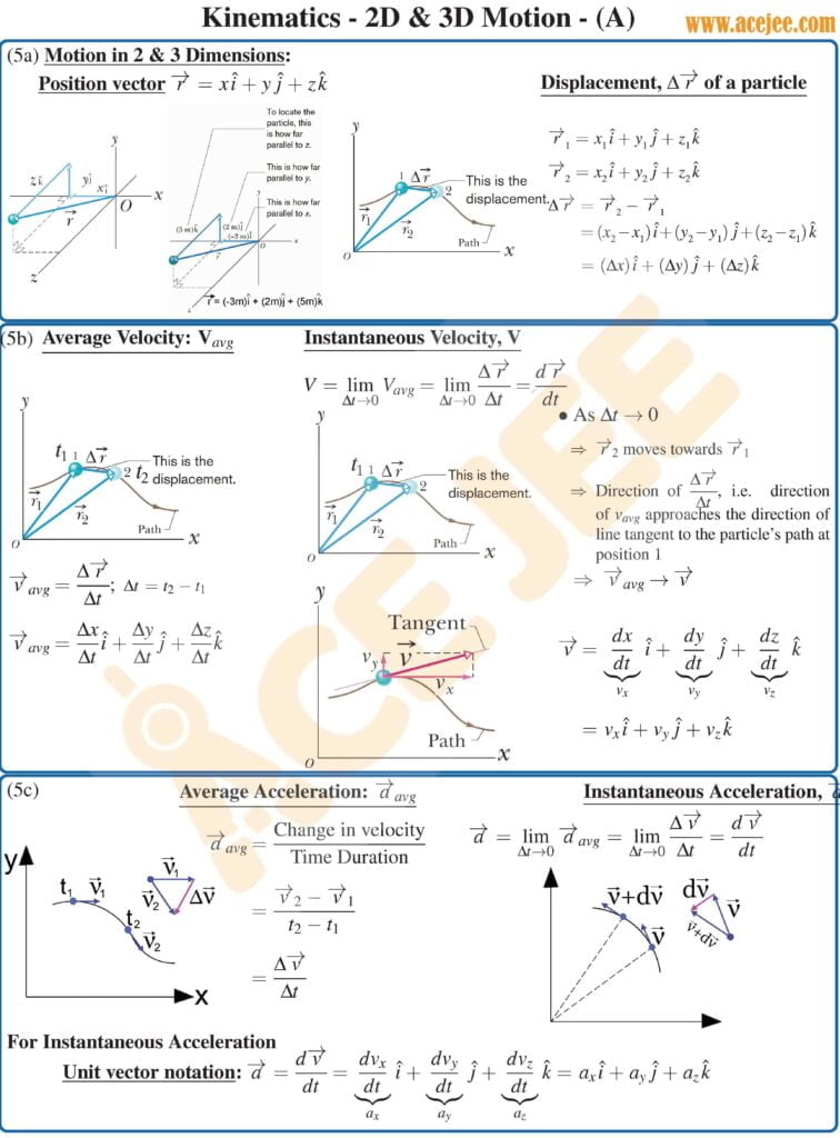
This provides the rigorous proof for a key concept from our last lesson: the velocity vector $v$ is always tangent to the particle's path. This is why, in the intrinsic coordinate system, we could define the tangential unit vector as $u^_{t} = \frac{v}{∣ v ∣}$ . The direction of velocity defines the tangent to the trajectory.

Conclusion

Today, we have rigorously established the definition of instantaneous velocity from first principles. By applying the concept of limits to the intuitive notion of average velocity, we arrived at the formal definition of the derivative.

Key Takeaways:

Average velocity $v ˉ = \frac{Δ x}{Δ t}$ is the slope of the secant line on a position-time graph.
Instantaneous velocity $v (t) = lim_{Δ t \to 0} \frac{Δ x}{Δ t} = \frac{d x}{d t}$ is the slope of the tangent line on a position-time graph.
In 3D, the instantaneous velocity vector $v (t) = \frac{d r}{d t}$ is always tangent to the particle's trajectory.

We have solidified the first crucial link in kinematics: the relationship between position and velocity. In our next lesson, we will apply this exact same logic one level higher. We will derive instantaneous acceleration from average acceleration using limits, establishing the complete differential relationship between position, velocity, and acceleration.

Recommended resources

1. The Inadequacy of Average Velocity

2. The Limiting Process: From Average to Instantaneous

3. The Geometric Interpretation: Slopes of Lines

4. Generalization to Three Dimensions

Conclusion