3D Angular Velocity and Acceleration in Spatial Motion

1. Angular Velocity as a True Vector

A fundamental question you might have is why we can treat angular velocity as a vector. After all, finite rotations are not commutative (rotating a book 90 degrees about the x-axis then 90 degrees about the y-axis gives a different result than performing the rotations in the reverse order), and vector addition must be commutative.

The answer lies in the transition from finite rotations to infinitesimal ones. While finite rotations are not vectors, infinitesimal rotations are. Since angular velocity is defined as the time rate of change of angular displacement, $\vec{\omega }=d\vec{\theta }/dt$, it inherits this vector property from infinitesimal rotations.

The key consequence of $\vec{\omega }$ being a true vector is that angular velocities add vectorially. If a body is subject to multiple simultaneous rotations, its instantaneous angular velocity is simply the vector sum of the individual angular velocities.

Example: A Spinning, Tumbling Globe
Imagine a globe spinning on its polar axis with angular velocity ${\vec{\omega }}_1$. Now, you tumble the entire assembly about a horizontal axis with angular velocity ${\vec{\omega }}_2$. The total instantaneous angular velocity of the globe is ${\vec{\omega }}_{\text{total}}={\vec{\omega }}_1+{\vec{\omega }}_2$. At any instant, the globe is rotating about a single effective axis defined by the direction of ${\vec{\omega }}_{\text{total}}$. The points on the globe that lie on this axis are instantaneously at rest (relative to the globe's center). This concept is explored in the "Mechanics VIII: 3D Rotation" handout (resource LINK), Example 1.

2. Angular Acceleration in 3D: The Concept of Precession

Angular acceleration is defined as the time derivative of the angular velocity vector:
$\vec{\alpha }=\frac{d\vec{\omega }}{dt}$
In 2D, this simply meant the rate of change of the spin speed. But in 3D, this definition is far more powerful. Since $\vec{\omega }$ is a vector, it can change in two ways:

1. Its magnitude can change (the object spins faster or slower).
2. Its direction can change (the axis of rotation tilts or turns).

Even if the angular speed $|\vec{\omega }|$ is constant, if the axis of rotation is turning, there will be a non-zero angular acceleration $\vec{\alpha }$. This motion, where the axis of angular velocity itself rotates, is called precession.

The angular velocity of the precession is denoted by $\vec{\Omega }$. The rate of change of $\vec{\omega }$ due to this precession is given by the cross product:
$\frac{d\vec{\omega }}{dt}=\vec{\Omega }\times \vec{\omega }$
This is a general result for the time derivative of any vector $\vec{A}$ that is rotating with an angular velocity $\vec{\Omega }$: $d\vec{A}/dt=\vec{\Omega }\times \vec{A}$.

In the most general case, where an object is both changing its spin rate and its axis is precessing, the total angular acceleration is:
$\vec{\alpha }=\frac{d\vec{\omega }}{dt}={\left(\frac{d\vec{\omega }}{dt}\right)}_{\text{body frame}}+\vec{\Omega }\times \vec{\omega }$
Here, the first term accounts for the change in magnitude of $\vec{\omega }$, and the second term accounts for the change in its direction.

3. Application: The Kinematics of a Precessing Gyroscope

The quintessential example of this phenomenon is a precessing gyroscope. While the full treatment involves dynamics (torque $\vec{\tau }$ and angular momentum $\vec{L}$), the core of the motion is kinematic. The relation $\vec{\tau }=d\vec{L}/dt$ dictates how the angular momentum vector changes. For a symmetric object spinning rapidly about its axis, $\vec{L}$ is approximately parallel to $\vec{\omega }$, so understanding the change in $\vec{L}$ tells us about the change in $\vec{\omega }$.

Let's watch a video that derives the motion from first principles. It beautifully illustrates how a torque perpendicular to the angular momentum causes a change in its direction, leading to precession.

The crucial kinematic insight from the video is that the change in the angular momentum vector, $d\vec{L}$, is perpendicular to $\vec{L}$ itself. This means the torque only changes the direction of $\vec{L}$, causing it to swing around in a circle—this is precession. The rate of this swing is the precessional angular velocity $\Omega$.

4. Problem-Solving with 3D Kinematic Vectors

Now, let's apply this vector-based approach to a problem of the type you might encounter in the JEE Advanced exam. These problems often require you to describe motion using 3D vectors and then perform vector operations.

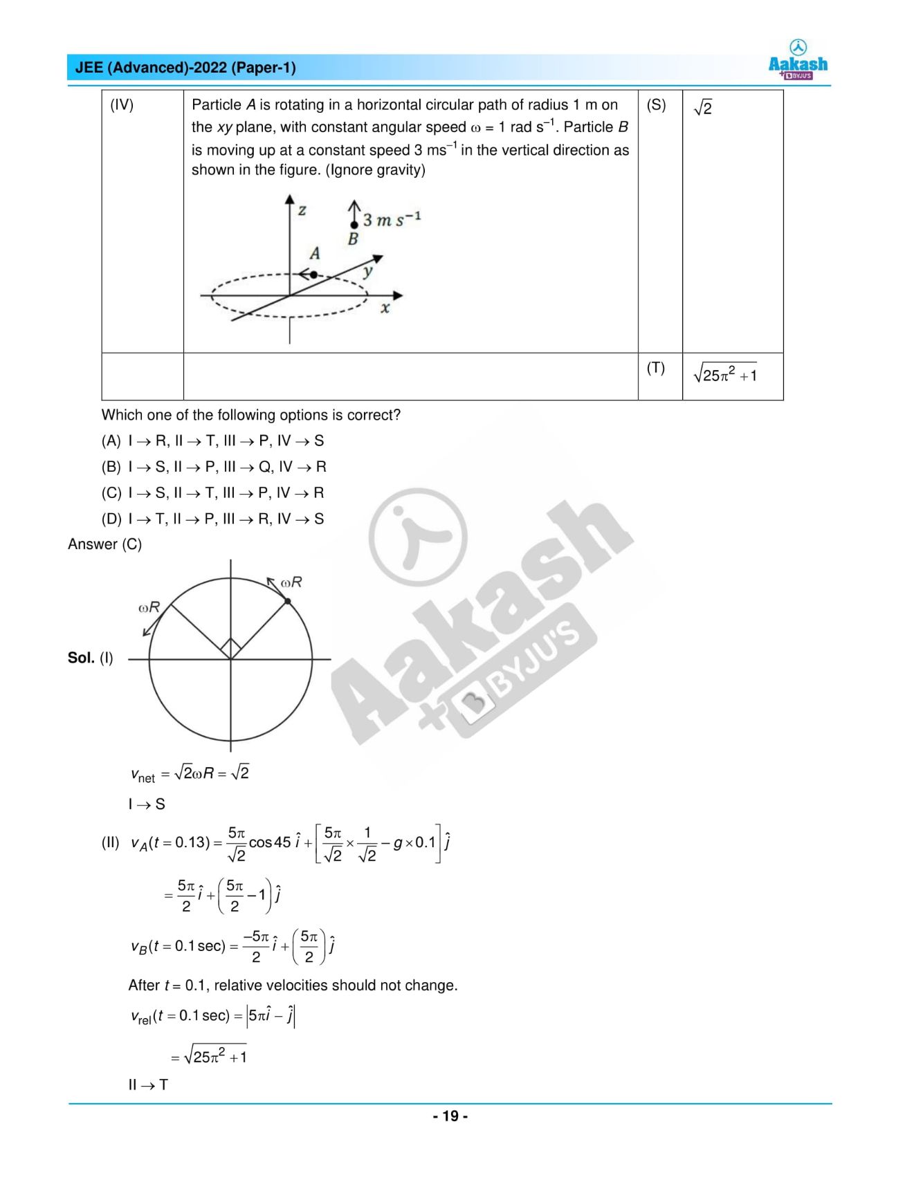
Let's break down this problem.

Given:

• Particle A: Uniform circular motion in the xy-plane.
  • Center at origin (0, 0, 0).
  • Radius $R=1/\pi$ m.
  • Angular speed $\omega =\pi$ rad/s.
  • At $t=0$, particle A is at $(R,0,0)$.
• Particle B: Constant velocity along the z-axis.
  • Velocity ${\vec{v}}_B=v_0\hat{k}$ with $v_0=3/2\pi$ m/s.
  • At $t=0$, particle B is at $(0,0,0)$.

The question asks to evaluate statements about the relative velocity at $t=0.5$ s.

Step 1: Write the position and velocity vectors for each particle.

• Particle A:
  The angular position at time $t$ is $\theta (t)=\omega t$. The position vector is:
  ${\vec{r}}_A(t)=R\cos (\omega t)\hat{i}+R\sin (\omega t)\hat{j}$
  The angular velocity vector is $\vec{\omega }=\omega \hat{k}$ (by the right-hand rule for counter-clockwise motion in the xy-plane). The velocity vector can be found either by differentiating ${\vec{r}}_A(t)$ or by using the cross product ${\vec{v}}_A=\vec{\omega }\times {\vec{r}}_A$. Let's use differentiation:
  ${\vec{v}}_A(t)=\frac{d{\vec{r}}_A}{dt}=-R\omega \sin (\omega t)\hat{i}+R\omega \cos (\omega t)\hat{j}$

• Particle B:
  The velocity is constant. The position vector is:
  ${\vec{r}}_B(t)=(v_{0}t)\hat{k}$
  The velocity vector is:
  ${\vec{v}}_B(t)=v_0\hat{k}$

This problem highlights that even for motions that seem simple when viewed independently, their combination in 3D space requires a systematic vector approach.

Conclusion

In this lesson, we have generalized our understanding of rotational kinematics to three dimensions. This required a deeper appreciation for the vector nature of angular quantities and the use of the cross product to describe how these vectors change over time.

Key Takeaways:

• Angular velocity $\vec{\omega }$ and angular acceleration $\vec{\alpha }$ are true vectors because infinitesimal rotations are commutative and can be added vectorially.
• The total instantaneous angular velocity of a body is the vector sum of its component angular velocities (e.g., spin + precession).
• Angular acceleration, $\vec{\alpha }=d\vec{\omega }/dt$, arises from a change in either the magnitude or the direction of the angular velocity vector.
• The change in direction of $\vec{\omega }$ is called precession and is described kinematically by the term $\vec{\Omega }\times \vec{\omega }$, where $\vec{\Omega }$ is the precession angular velocity.
• Solving problems in spatial motion requires consistently representing all kinematic quantities as 3D vectors and using the rules of vector algebra and calculus.

Preview of the Next Module:
We have now completed our deep dive into the kinematics of a single rigid body. The vector tools you've honed here are indispensable for the next stage of our course. The next module, Relative Motion, will focus on describing and analyzing the motion of objects from different, moving reference frames. The rigorous derivation of transformations between frames, especially rotating ones, builds directly on the 3D vector kinematics we've studied today.