Connecting Linear and Angular Motion

1. Angular Quantities as Vectors

Before we can prove the relationships, we must first formally define angular velocity and acceleration as vector quantities.

• Angular Velocity ($\vec{\omega }$):

  • Magnitude: The magnitude $|\vec{\omega }|=\omega$ is the angular speed, i.e., the rate of change of the angle, $\omega =|d\theta /dt|$.
  • Direction: The vector $\vec{\omega }$ points along the axis of rotation. Its specific direction is determined by the right-hand thumb rule: if you curl the fingers of your right hand in the direction of rotation, your thumb points in the direction of $\vec{\omega }$.

• Angular Acceleration ($\vec{\alpha }$):

  • Definition: The angular acceleration vector is the time derivative of the angular velocity vector: $\vec{\alpha }=d\vec{\omega }/dt$.
  • Direction: If the rotation is speeding up (i.e., $\omega$ is increasing), $\vec{\alpha }$ points in the same direction as $\vec{\omega }$. If the rotation is slowing down, $\vec{\alpha }$ points in the opposite direction.

The following video provides an excellent visual introduction to these concepts and asserts the vector relationships we are about to prove.

2. The Calculus of a Rotating Frame

The core challenge in deriving the link between linear and angular velocity lies in the fact that for a rotating object, the natural coordinate system (polar or cylindrical) has unit vectors that themselves change direction over time. A Cartesian system with fixed $\hat{i}$ and $\hat{j}$ vectors does not have this complexity ($d\hat{i}/dt=0$), but it is less natural for describing rotation.

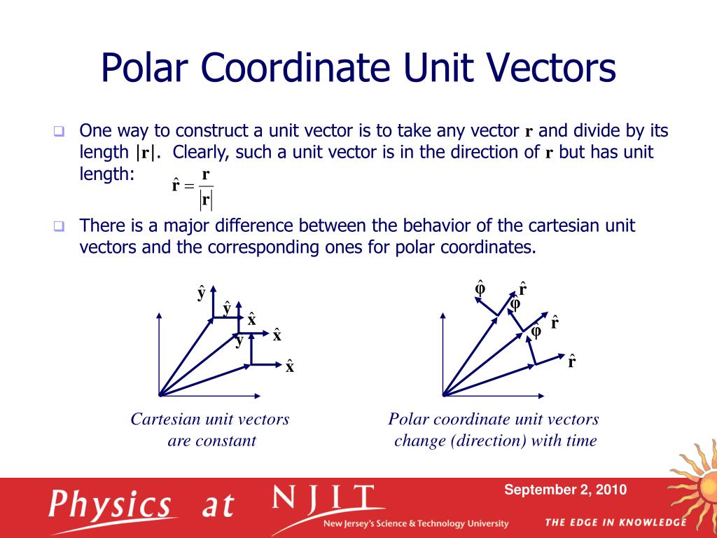
To derive the velocity, we must differentiate the position vector $\vec{r}$. In polar coordinates, the position of a particle is elegantly expressed as:
$\vec{r}(t)=r(t){\hat{u}}_r(t)$
where $r(t)$ is the radial distance from the origin and ${\hat{u}}_r(t)$ is the radial unit vector.

3. Proof: The Relationship between Linear and Angular Velocity

To find the velocity $\vec{v}=d\vec{r}/dt$, we apply the product rule:
$\vec{v}=\frac{d}{dt}[r(t){\hat{u}}_r(t)]=\frac{dr}{dt}{\hat{u}}_r+r\frac{d{\hat{u}}_r}{dt}$
The term $\frac{dr}{dt}{\hat{u}}_r$ represents the velocity component due to a change in the radial distance. The term $r\frac{d{\hat{u}}_r}{dt}$ arises from the rotation of the position vector. The key is to evaluate $d{\hat{u}}_r/dt$.

The following resource provides a rigorous, step-by-step derivation of the velocity vector in polar coordinates by first finding the time derivatives of the polar unit vectors. This is a fundamental proof that underpins much of rotational mechanics.

As you saw in the reading, the derivation shows that $d{\hat{u}}_r/dt=\omega {\hat{u}}_{\theta }$. For circular motion, the radius $r$ is constant, so $dr/dt=0$. The velocity expression simplifies to:
$\vec{v}=r\omega {\hat{u}}_{\theta }$
This equation states that the velocity vector has a magnitude of $r\omega$ and points in the tangential direction ${\hat{u}}_{\theta }$.

Now, let's prove this is identical to the cross product $\vec{\omega }\times \vec{r}$.
Consider motion in the $xy$-plane, with the axis of rotation along the $z$-axis.

• $\vec{\omega }=\omega \hat{k}$
• $\vec{r}=r{\hat{u}}_r=r(\cos \theta \hat{i}+\sin \theta \hat{j})$

Let's compute the cross product:
$\vec{\omega }\times \vec{r}=(\omega \hat{k})\times [r(\cos \theta \hat{i}+\sin \theta \hat{j})]=r\omega [\cos \theta (\hat{k}\times \hat{i})+\sin \theta (\hat{k}\times \hat{j})]$
Using the cyclic property of unit vector cross products ($\hat{k}\times \hat{i}=\hat{j}$ and $\hat{k}\times \hat{j}=-\hat{i}$):
$\vec{\omega }\times \vec{r}=r\omega [\cos \theta (\hat{j})+\sin \theta (-\hat{i})]=r\omega (-\sin \theta \hat{i}+\cos \theta \hat{j})$
Recognizing that the term in the parenthesis is the definition of the tangential unit vector ${\hat{u}}_{\theta }$, we have:
$\vec{\omega }\times \vec{r}=r\omega {\hat{u}}_{\theta }$
This is identical to the result from our differentiation, thus proving the fundamental relationship for circular motion:
$\vec{v}=\vec{\omega }\times \vec{r}$

4. Proof: The Relationship between Linear and Angular Acceleration

Having established $\vec{v}=\vec{\omega }\times \vec{r}$, we can find the acceleration $\vec{a}$ by differentiating $\vec{v}$ with respect to time. We use the product rule for cross products, remembering that both $\vec{\omega }$ (in non-uniform motion) and $\vec{r}$ can change with time.

$\vec{a}=\frac{d\vec{v}}{dt}=\frac{d}{dt}(\vec{\omega }\times \vec{r})=\left(\frac{d\vec{\omega }}{dt}\times \vec{r}\right)+\left(\vec{\omega }\times \frac{d\vec{r}}{dt}\right)$

Let's analyze the two resulting terms:

1. First term: $\left(\frac{d\vec{\omega }}{dt}\times \vec{r}\right)$
   By definition, $\frac{d\vec{\omega }}{dt}=\vec{\alpha }$, the angular acceleration. So this term is $\vec{\alpha }\times \vec{r}$.

   • Direction: $\vec{\alpha }$ is along the axis of rotation (e.g., $\hat{k}$), and $\vec{r}$ is in the plane of rotation. Their cross product, by the right-hand rule, points along the tangent (${\hat{u}}_{\theta }$).
   • Magnitude: $|\vec{\alpha }\times \vec{r}|=|\vec{\alpha }||\vec{r}|\sin (90^{\circ })=\alpha r$.
     This term is exactly the tangential acceleration, ${\vec{a}}_t$, which changes the magnitude of the velocity. This proves our second learning outcome:
     ${\vec{a}}_t=\vec{\alpha }\times \vec{r}$

2. Second term: $\left(\vec{\omega }\times \frac{d\vec{r}}{dt}\right)$
   We know that $\frac{d\vec{r}}{dt}=\vec{v}$. So this term is $\vec{\omega }\times \vec{v}$.
   Since $\vec{v}=\vec{\omega }\times \vec{r}$, this term becomes $\vec{\omega }\times (\vec{\omega }\times \vec{r})$.
   This term is the centripetal acceleration, ${\vec{a}}_c$.
   To understand its properties, we use the vector triple product identity: $\vec{A}\times (\vec{B}\times \vec{C})=\vec{B}(\vec{A}\cdot \vec{C})-\vec{C}(\vec{A}\cdot \vec{B})$.
   ${\vec{a}}_c=\vec{\omega }\times (\vec{\omega }\times \vec{r})=\vec{\omega }(\vec{\omega }\cdot \vec{r})-\vec{r}(\vec{\omega }\cdot \vec{\omega })$
   For circular motion in a plane, $\vec{\omega }$ is perpendicular to $\vec{r}$, so their dot product $\vec{\omega }\cdot \vec{r}=0$. The expression simplifies dramatically:
   ${\vec{a}}_c=0-\vec{r}({\omega }^2)=-{\omega }^2\vec{r}$

   • Direction: The negative sign shows that the acceleration is in the opposite direction to the position vector $\vec{r}$, meaning it points radially inward, towards the center.
   • Magnitude: $|{\vec{a}}_c|=|-{\omega }^2\vec{r}|={\omega }^{2}r$.
     This perfectly matches our formula for centripetal acceleration.

Combining the two components, we arrive at the complete vector expression for acceleration in circular motion:
$\vec{a}={\vec{a}}_t+{\vec{a}}_c=(\vec{\alpha }\times \vec{r})+(\vec{\omega }\times (\vec{\omega }\times \vec{r}))$

Conclusion

In this lesson, we have moved from scalar descriptions to a more powerful and general vector framework for circular motion. Through rigorous, calculus-based proofs, we have established the fundamental connections between linear and angular kinematic quantities.

Key Takeaways:

• Angular velocity ($\vec{\omega }$) and angular acceleration ($\vec{\alpha }$) are axial vectors, with directions defined by the right-hand rule.
• The linear velocity $\vec{v}$ of a point on a rotating body is given by the cross product $\vec{v}=\vec{\omega }\times \vec{r}$.
• The total linear acceleration $\vec{a}$ has two components derived from differentiating the velocity vector:
  • Tangential Acceleration: ${\vec{a}}_t=\vec{\alpha }\times \vec{r}$, which arises from a change in angular speed.
  • Centripetal Acceleration: ${\vec{a}}_c=\vec{\omega }\times (\vec{\omega }\times \vec{r})=-{\omega }^2\vec{r}$, which arises from the change in the direction of velocity.

Preview of the Next Lesson:
Now that we have rigorously derived the differential relationships connecting position, velocity, and acceleration in rotation, we are equipped to solve a wider class of problems. In the next lesson, we will focus on cases where the angular acceleration $\alpha$ is not constant but varies with time, $\alpha (t)$. This will require us to use integration to find the angular velocity $\omega$ and angular position $\theta$ as functions of time.