Deriving Kinematic Equations from Calculus

Hello! Welcome to the first lesson of Module 2.

In our previous module, we established the fundamental differential relationships of kinematics from first principles. We proved that velocity is the time derivative of position ( $v = d r / d t$ ) and acceleration is the time derivative of velocity ( $a = d v / d t$ ). Your preference for rigorous proofs was key to building that solid foundation.

Today, we will leverage that foundation to achieve this lesson's learning outcome: to derive the set of kinematic equations for constant acceleration from first principles using calculus. We will reverse the process of differentiation through integration, applying the crucial condition that acceleration is constant. This special case is not only fundamental to physics but also a cornerstone of problems you will encounter in your JEE Advanced preparation.

1. The Principle of Derivation: Integration

Recall the two fundamental differential equations of one-dimensional motion:

$a = \frac{d v}{d t}$
$v = \frac{d x}{d t}$

If acceleration $a$ is not constant but a function of time, $a (t)$ , these remain differential equations that must be solved. However, a very important special case in mechanics is when acceleration is constant. In this scenario, we can integrate these equations directly to find expressions for velocity and position as functions of time.

Our method will be to use definite integrals. This is a mathematically rigorous way to incorporate the "initial conditions" of the motion—the state of the object at time $t = 0$ .

2. Derivation 1: Velocity as a Function of Time

We begin with the definition of acceleration:

a = \frac{d v}{d t}

Our core assumption is that $a$ is a constant. To find the velocity $v$ at some arbitrary time $t$ , we can integrate. First, we separate the variables, placing all velocity-related terms on one side and time-related terms on the other:

d v = a d t

Now, we integrate both sides. We integrate velocity from its initial value, which we'll call $v_{0}$ (or $u$ ), to its final value $v$ . Simultaneously, we integrate time from the start, $t = 0$ , to the final time $t$ .

\int_{v_{0}}^{v} d v = \int_{0}^{t} a d t

Since $a$ is constant, we can move it outside the integral on the right-hand side:

\int_{v_{0}}^{v} d v = a \int_{0}^{t} d t

Evaluating these simple integrals gives:

[v]_{v_{0}}^{v} = a [t]_{0}^{t}

v - v_{0} = a (t - 0)

Rearranging this gives us the first kinematic equation:

v = v_{0} + a t

3. Derivation 2: Position as a Function of Time

Next, we start with the definition of velocity:

v = \frac{d x}{d t}

We can now substitute the expression for $v (t)$ that we just derived:

\frac{d x}{d t} = v_{0} + a t

Again, we separate variables to prepare for integration:

d x = (v_{0} + a t) d t

We integrate both sides. Position is integrated from its initial value $x_{0}$ to its final value $x$ . Time is integrated from $0$ to $t$ .

\int_{x_{0}}^{x} d x = \int_{0}^{t} (v_{0} + a t) d t

The integral on the left is straightforward. The integral on the right can be split into two parts:

[x]_{x_{0}}^{x} = \int_{0}^{t} v_{0} d t + \int_{0}^{t} a t d t

Since $v_{0}$ and $a$ are constants:

x - x_{0} = v_{0} \int_{0}^{t} d t + a \int_{0}^{t} t d t

Evaluating the integrals yields:

x - x_{0} = v_{0} [t]_{0}^{t} + a [\frac{t ^{2}}{2}]_{0}^{t}

x - x_{0} = v_{0} t + \frac{1}{2} a t^{2}

This is our second kinematic equation. The term $x - x_{0}$ represents the displacement, often denoted by $s$ or $Δ x$ .

4. Derivation 3: The Time-Independent Equation

For the third core equation, we could simply eliminate time $t$ algebraically between the first two equations. However, a more elegant and powerful method, which you'll find useful in more advanced problems, involves a "trick" using the chain rule. This method avoids direct reference to time.

We start again with $a = \frac{d v}{d t}$ . Using the chain rule, we can write this as:

a = \frac{d v}{d x} \cdot \frac{d x}{d t}

Since we know that $v = \frac{d x}{d t}$ , we can substitute this in:

a = v \frac{d v}{d x}

This relationship, $a = v \frac{d v}{d x}$ , is extremely useful and will be the key to solving problems with position-dependent acceleration later in this course.

Now, we separate variables, putting all velocity terms with $d v$ and all position terms with $d x$ :

v d v = a d x

We integrate both sides. Velocity is integrated from $v_{0}$ to $v$ , and position from $x_{0}$ to $x$ :

\int_{v_{0}}^{v} v d v = \int_{x_{0}}^{x} a d x

Since $a$ is constant:

\int_{v_{0}}^{v} v d v = a \int_{x_{0}}^{x} d x

Evaluating these integrals gives:

[\frac{v ^{2}}{2}]_{v_{0}}^{v} = a [x]_{x_{0}}^{x}

\frac{v ^{2}}{2} - \frac{v _{0}^{2}}{2} = a (x - x_{0})

Multiplying by 2 and rearranging gives the third kinematic equation:

v^{2} = v_{0}^{2} + 2 a (x - x_{0})

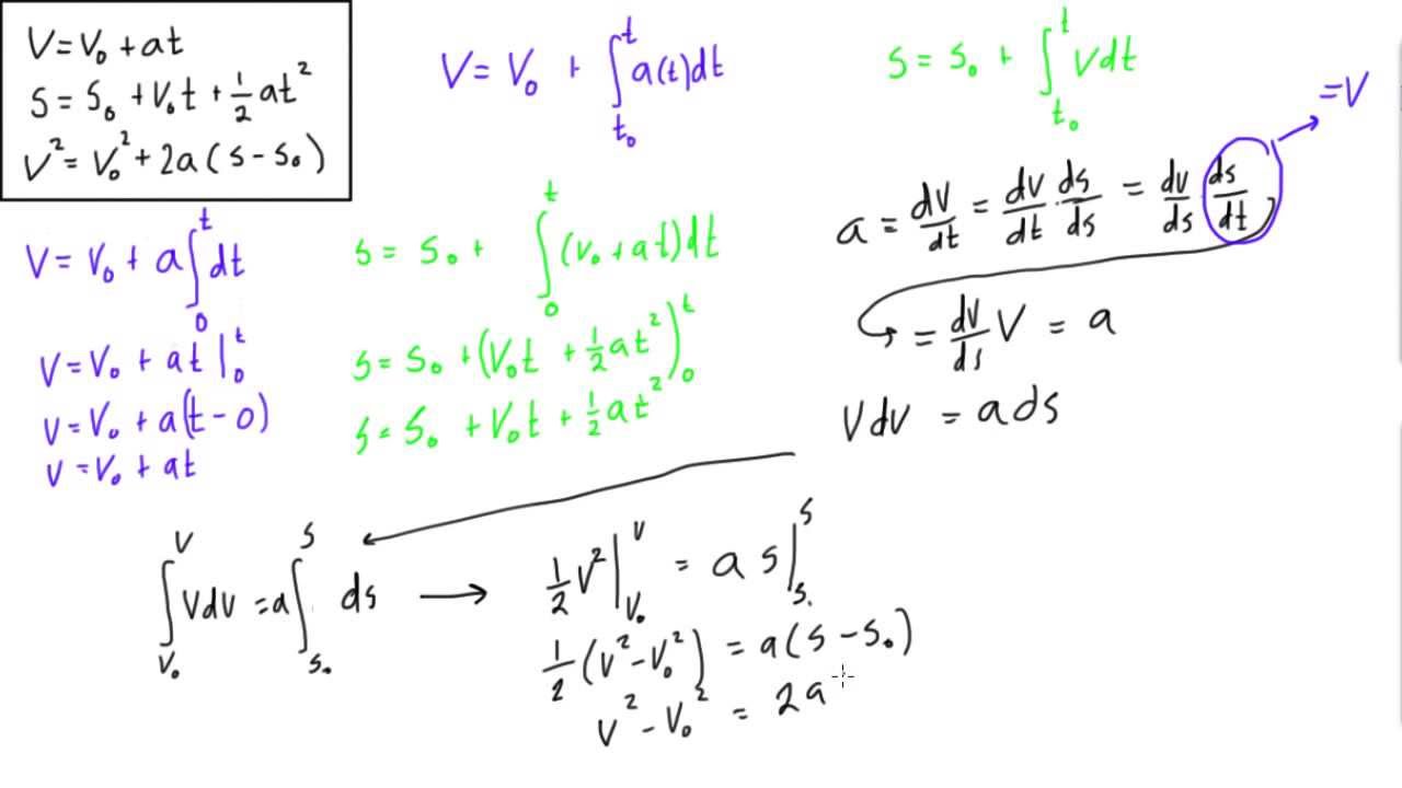
The following document provides a concise, formal summary of these three derivations, which aligns with your preference for rigorous mathematical arguments.

Kinematics and Calculus

The resource 'Kinematics and Calculus' from The Physics Hypertextbook provides a sharp, calculus-based derivation of the three main kinematic equations. Pay special attention to the clever chain-rule method used for the third equation.

Read the entire section under the heading 'motion with constant acceleration'. It walks through the three derivations we just discussed. Note how it frames the derivation of the third equation as a 'sophisticated trick', highlighting its elegance.

The image below provides a clean, visual summary of the three calculus-based derivations we have just performed.

Derivation of Kinematic Equations using Calculus — This image summarizes the derivation of the three core kinematic equations for constant acceleration from the first principles of calculus: integrating $a=dv/dt$ to get $v(t)$, integrating $v(t)=dx/dt$ to get $x(t)$, and integrating $a=v(dv/dx)$ to get the time-independent equation.

Test your understanding!

In our first derivation, we took the equation $\int_{v_{0}}^{v} d v = \int_{0}^{t} a d t$ and simplified it to $\int_{v_{0}}^{v} d v = a \int_{0}^{t} d t$ .

What specific assumption allows us to move the term a outside the integral?
If the acceleration were given by $a (t) = k t$ , where $k$ is a constant, could we still make this step? What would the resulting equation for velocity be?

Show answer

We can only move $a$ outside the integral because we have assumed it is constant with respect to the variable of integration, time ( $t$ ). If $a$ were a function of time, it could not be treated as a constant factor. This is the precise mathematical step where the "constant acceleration" condition is enforced.
No, we could not make that step. We would have to evaluate the integral $\int_{0}^{t} k t d t$ . The resulting derivation would be: $v - v_{0} = \int_{0}^{t} k t d t = k [\frac{t ^{2}}{2}]_{0}^{t} = \frac{1}{2} k t^{2}$ So, the velocity would be $v (t) = v_{0} + \frac{1}{2} k t^{2}$ . This demonstrates how the calculus method naturally handles non-constant acceleration, a topic we will explore in the next lessons.

5. Completing the Set: The Algebraic Derivations

For problem-solving, particularly in timed exams like the JEE, it's useful to have a full set of five equations. The remaining two are not independent but are derived algebraically from the first two fundamental equations we proved with calculus.

$v = v_{0} + a t (1)$
$Δ x = v_{0} t + \frac{1}{2} a t^{2} (2)$

The following video demonstrates how to derive these, along with the other equations, providing a complete picture. While we have focused on the more rigorous calculus proofs, seeing the algebraic connections is also valuable.

Deriving the Kinematic Equations of Motion w/ Constant Acceleration in Physics - [1-2-13]

The video 'Deriving the Kinematic Equations of Motion' by Math and Science walks through the derivation of all five common kinematic equations. We've already rigorously derived the main three using a more formal calculus approach. You can watch the indicated sections to see how the final two equations are derived through algebraic substitution.

Watch the segments from 14:01 to 17:02 (deriving Δx = vt - ½at²) and from 17:02 to 19:54 (deriving Δx = ½(v₀+v)t). Notice that these are purely algebraic manipulations of the first two equations.

Here is the full set of five equations, often called the "SUVAT" equations in some contexts (where $s$ is displacement, $u$ is initial velocity, $v$ is final velocity, $a$ is acceleration, $t$ is time):

$v = u + a t$
$s = u t + \frac{1}{2} a t^{2}$
$v^{2} = u^{2} + 2 a s$
$s = v t - \frac{1}{2} a t^{2}$
$s = \frac{1}{2} (u + v) t$

Conclusion

In this lesson, you have seen how the kinematic equations, which you may have previously memorized, are not arbitrary formulas but are direct mathematical consequences of integrating the definitions of velocity and acceleration under the condition of constant acceleration.

Key Takeaways:

The three core kinematic equations can be derived rigorously from first principles using definite integration.
The equation $v = v_{0} + a t$ comes from integrating $a = d v / d t$ .
The equation $Δ x = v_{0} t + \frac{1}{2} a t^{2}$ comes from integrating $v = d x / d t$ .
The time-independent equation $v^{2} = v_{0}^{2} + 2 a Δ x$ is elegantly derived using the chain rule identity $a = v \frac{d v}{d x}$ .
The full set of five equations is completed by algebraic manipulation.
Crucially, these equations are only valid when acceleration is constant.

Preview of the Next Lesson:

Now that we have mastered the special case of constant acceleration, we will return to the more general situation. In the next lesson, you will learn how to solve problems with time-dependent acceleration, $a (t)$ , by applying the same method of direct integration. This will further solidify your understanding of the power and generality of the calculus approach to kinematics.