Deconstructing 2D Motion: The Principle of Independence

1. From Scalars to Vectors: Describing 2D Motion

In one-dimensional motion, we could represent position, velocity, and acceleration with scalars (e.g., $x(t)$, $v(t)$, $a(t)$), where the sign indicated direction. For motion in a plane or in space, this is no longer sufficient. We must use vectors to capture both magnitude and direction.

The fundamental kinematic quantities are now vectors:

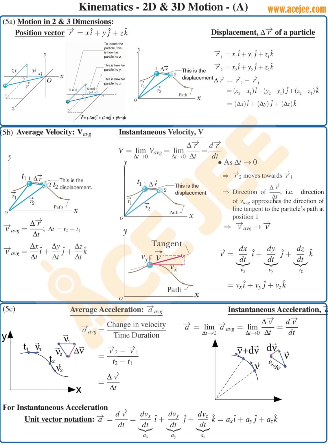
• Position Vector: $\vec{r}(t)$ - A vector from the origin of our coordinate system to the particle's location at time $t$.
• Velocity Vector: $\vec{v}(t)$ - The rate of change of the position vector.
• Acceleration Vector: $\vec{a}(t)$ - The rate of change of the velocity vector.

The image below gives a comprehensive overview of these vector quantities in a 3D context. The same ideas apply directly to 2D motion.

2. The Proof: Independence of Perpendicular Motion

Our goal is to prove that motion along one axis (e.g., the x-axis) is entirely independent of the motion along a perpendicular axis (e.g., the y-axis). The entire proof hinges on the properties of vector differentiation in a fixed coordinate system.

Let's establish a standard 2D Cartesian coordinate system with a fixed origin and constant, perpendicular unit vectors $\hat{i}$ and $\hat{j}$.

The position vector of a particle at any time $t$ can be written in terms of its components:
$\vec{r}(t)=x(t)\hat{i}+y(t)\hat{j}$

Step 1: Deriving the Velocity Vector

By definition, the instantaneous velocity vector $\vec{v}(t)$ is the time derivative of the position vector $\vec{r}(t)$.
$\vec{v}(t)=\frac{d\vec{r}}{dt}=\frac{d}{dt}\left(x(t)\hat{i}+y(t)\hat{j}\right)$
Using the product rule for differentiation on each term:
$\vec{v}(t)=\left(\frac{dx}{dt}\hat{i}+x(t)\frac{d\hat{i}}{dt}\right)+\left(\frac{dy}{dt}\hat{j}+y(t)\frac{d\hat{j}}{dt}\right)$
Here is the critical step: since our coordinate system is fixed (non-rotating and non-accelerating), the basis vectors $\hat{i}$ and $\hat{j}$ are constant in both magnitude and direction. Therefore, their time derivatives are zero:
$\frac{d\hat{i}}{dt}=0\text{and}\frac{d\hat{j}}{dt}=0$
This simplifies the velocity vector equation to:
$\vec{v}(t)=\frac{dx}{dt}\hat{i}+\frac{dy}{dt}\hat{j}$
If we define the components of the velocity vector as $\vec{v}(t)=v_x(t)\hat{i}+v_y(t)\hat{j}$, we see by direct comparison that:
$v_x(t)=\frac{dx}{dt}\text{and}{v}_y(t)=\frac{dy}{dt}$
This result is the first part of our proof. It shows that the x-component of velocity, $v_x$, depends only on the rate of change of the x-position, $x(t)$. It is completely unaffected by $y(t)$ or $v_y(t)$. The same is true for the y-component.

Step 2: Deriving the Acceleration Vector

The same logic applies to acceleration, which is the time derivative of velocity:
$\vec{a}(t)=\frac{d\vec{v}}{dt}=\frac{d}{dt}\left(v_x(t)\hat{i}+v_y(t)\hat{j}\right)$
Again, because $\hat{i}$ and $\hat{j}$ are constant, the derivative passes through to the scalar components:
$\vec{a}(t)=\frac{d{v}_x}{dt}\hat{i}+\frac{d{v}_y}{dt}\hat{j}$
Defining the components of acceleration as $\vec{a}(t)=a_x(t)\hat{i}+a_y(t)\hat{j}$, we find:
$a_x(t)=\frac{d{v}_x}{dt}=\frac{d^{2}x}{d{t}^2}\text{and}{a}_y(t)=\frac{d{v}_y}{dt}=\frac{d^{2}y}{d{t}^2}$
This completes the proof. The x-component of acceleration depends only on the x-component of velocity, and the y-component of acceleration depends only on the y-component of velocity.

Conclusion of the Proof:
We have mathematically demonstrated that the kinematic equations along the x-axis ($a_x=d{v}_x/dt$, $v_x=dx/dt$) and the y-axis ($a_y=d{v}_y/dt$, $v_y=dy/dt$) form two independent sets of differential equations. The only variable that connects them is time, $t$. This is the Principle of Independence of Motion.

The following resource provides an excellent summary of these derivations.

3. A Visual Demonstration

The principle can be counter-intuitive at first. A classic thought experiment provides powerful visual evidence. Imagine two balls at the top of a building. One is dropped straight down, and the other is launched horizontally at the same instant.

As the image shows, if we ignore air resistance, both balls hit the ground at the same time. The horizontal velocity of the yellow ball has zero effect on its vertical motion. The vertical motion is governed solely by gravity, just as it is for the red ball. This is a perfect physical illustration of our mathematical proof.

4. Application to a General 2D Trajectory

Now, let's apply this principle. Consider a particle moving with a constant acceleration $\vec{a}=a_x\hat{i}+a_y\hat{j}$. Its initial velocity is ${\vec{v}}_0=v_{0x}\hat{i}+v_{0y}\hat{j}$ and initial position is ${\vec{r}}_0=x_0\hat{i}+y_0\hat{j}$.

Instead of trying to solve a complex 2D problem, we create two independent 1D problems:

X-Motion:

• Initial position: $x_0$
• Initial velocity: $v_{0x}$
• Acceleration: $a_x$ (constant)

From Module 2, we know the solutions are:

1. $v_x(t)=v_{0x}+a_{x}t$
2. $x(t)=x_0+v_{0x}t+\frac{1}{2}{a}_x{t}^2$

Y-Motion:

• Initial position: $y_0$
• Initial velocity: $v_{0y}$
• Acceleration: $a_y$ (constant)

The solutions are:

1. $v_y(t)=v_{0y}+a_{y}t$
2. $y(t)=y_0+v_{0y}t+\frac{1}{2}{a}_y{t}^2$

To find the particle's overall state at time $t$, we simply recombine the components:

• Velocity Vector: $\vec{v}(t)=(v_{0x}+a_{x}t)\hat{i}+(v_{0y}+a_{y}t)\hat{j}$
• Position Vector: $\vec{r}(t)=(x_0+v_{0x}t+\frac{1}{2}{a}_x{t}^2)\hat{i}+(y_0+v_{0y}t+\frac{1}{2}{a}_y{t}^2)\hat{j}$

Notice how these can be written in a compact vector form that mirrors the 1D equations:
$\vec{v}(t)={\vec{v}}_0+\vec{a}t$
$\vec{r}(t)={\vec{r}}_0+{\vec{v}}_{0}t+\frac{1}{2}\vec{a}{t}^2$
This demonstrates that the vector kinematic equations are simply a shorthand for the independent component-wise motions.

Worked Example

A particle starts from the origin (${\vec{r}}_0=\vec{0}$) at $t=0$ with an initial velocity ${\vec{v}}_0=(4.0\hat{i}-5.0\hat{j})$ m/s. It moves in the xy-plane with a constant acceleration $\vec{a}=(2.0\hat{i}+3.0\hat{j})$ m/s².

(a) Find the velocity vector at $t=3.0$ s.
We analyze the components independently:

• $v_x(3)=v_{0x}+a_{x}t=4.0+(2.0)(3.0)=10.0$ m/s
• $v_y(3)=v_{0y}+a_{y}t=-5.0+(3.0)(3.0)=4.0$ m/s
  So, $\vec{v}(3.0\text{ s})=(10.0\hat{i}+4.0\hat{j})$ m/s.

(b) Find the position vector at $t=3.0$ s.
Again, we use the component equations:

• $x(3)=x_0+v_{0x}t+\frac{1}{2}{a}_x{t}^2=0+(4.0)(3.0)+\frac{1}{2}(2.0)(3.0{)}^2=12.0+9.0=21.0$ m
• $y(3)=y_0+v_{0y}t+\frac{1}{2}{a}_y{t}^2=0+(-5.0)(3.0)+\frac{1}{2}(3.0)(3.0{)}^2=-15.0+13.5=-1.5$ m
  So, $\vec{r}(3.0\text{ s})=(21.0\hat{i}-1.5\hat{j})$ m.

Conclusion

Today, you have rigorously proven the foundational principle for all multidimensional kinematics.

Key Takeaways:

• Motion in two or three dimensions is described by vector quantities: position $\vec{r}(t)$, velocity $\vec{v}(t)$, and acceleration $\vec{a}(t)$.
• The Principle of Independence of Motion states that motion along perpendicular axes can be analyzed as separate, independent 1D problems.
• The proof of this principle rests on the fact that the basis vectors of a fixed Cartesian coordinate system are constant, allowing the time derivative operator to act on vector components independently.
• This principle allows us to solve complex 2D motion problems by applying the familiar 1D kinematic equations to each component separately.

Preview of the Next Lesson:
We will immediately apply this powerful principle to the most important case of 2D motion: projectile motion. By setting the acceleration to be constant and directed purely in the vertical direction ($\vec{a}=-g\hat{j}$), we will derive the parametric equations of motion, $x(t)$ and $y(t)$, that describe the path of any projectile.