Analyzing Trajectories in Non-Inertial Frames

1. The View from a Falling Object: Projectile Motion Re-examined

Let's begin with a classic, elegant scenario that is a staple of advanced physics problems. Imagine two particles, P1 and P2, are launched simultaneously and are only subject to gravity. What is the trajectory of P1 as observed by an observer on P2?

This is a question about relative motion, but between two accelerating objects. Let's analyze it from first principles using the tools we've derived.

• Inertial Frame (S, the ground): Both particles are projectiles. Their accelerations are constant and equal to the acceleration due to gravity, $\vec{g}$.

  • Acceleration of P1: ${\vec{a}}_1=\vec{g}$
  • Acceleration of P2: ${\vec{a}}_2=\vec{g}$

• Non-Inertial Frame (S', attached to P2): We place our observer on P2. This frame is accelerating along with P2.

  • Acceleration of the frame S': $\vec{A}={\vec{a}}_2=\vec{g}$.
  • We want to find the acceleration of P1 as measured in S', which we'll call ${\overrightarrow{a^{\prime }}}_{1\text{ rel }2}$.

Now, we apply the acceleration transformation equation we derived:
${\vec{a}}_1=\vec{A}+{\overrightarrow{a^{\prime }}}_{1\text{ rel }2}$

Substituting the known values:
$\vec{g}=\vec{g}+{\overrightarrow{a^{\prime }}}_{1\text{ rel }2}$

The immediate and profound conclusion is:
${\overrightarrow{a^{\prime }}}_{1\text{ rel }2}=\vec{0}$

Interpretation: The acceleration of one projectile relative to another is zero.

To an observer on projectile P2, projectile P1 appears to move with constant velocity. The trajectory is not a parabola, but a straight line. The velocity of this straight-line motion is the constant relative velocity, ${\overrightarrow{v^{\prime }}}_{1\text{ rel }2}={\vec{u}}_1-{\vec{u}}_2$, where ${\vec{u}}_1$ and ${\vec{u}}_2$ are their initial velocities.

This is a remarkable simplification. A problem involving two parabolic paths in an inertial frame becomes a problem of uniform linear motion in a non-inertial frame.

2. Application: Minimum Separation Between Two Projectiles

This principle is not just a theoretical curiosity; it's a powerful problem-solving technique. Let's apply it to a classic problem that becomes much simpler from a non-inertial perspective.

The video demonstrates that by switching to the reference frame of one of the projectiles, a complex kinematic problem involving two time-varying position vectors is reduced to a static geometry problem. This is the essence of applying our transformation equations to analyze trajectories.

3. The Dynamical Viewpoint: The Role of Fictitious Forces

We arrived at ${\overrightarrow{a^{\prime }}}_{1\text{ rel }2}=\vec{0}$ using kinematics. Let's verify this result from a dynamical perspective, using the concept of fictitious forces. An observer in the non-inertial frame S' (attached to P2) analyzes the forces acting on P1 to determine its acceleration ${\overrightarrow{a^{\prime }}}_{1\text{ rel }2}$.

According to this observer, the effective net force on P1 is the sum of all real forces and all fictitious forces:
${\overrightarrow{F^{\prime }}}_{\text{net}}={\vec{F}}_{\text{real}}+{\vec{F}}_{\text{fictitious}}$

• The only real force acting on P1 is gravity: ${\vec{F}}_{\text{real}}=m_1\vec{g}$.
• The fictitious force arises because the frame S' is accelerating with $\vec{A}=\vec{g}$. The fictitious force is ${\vec{F}}_{\text{fictitious}}=-m_1\vec{A}=-m_1\vec{g}$.

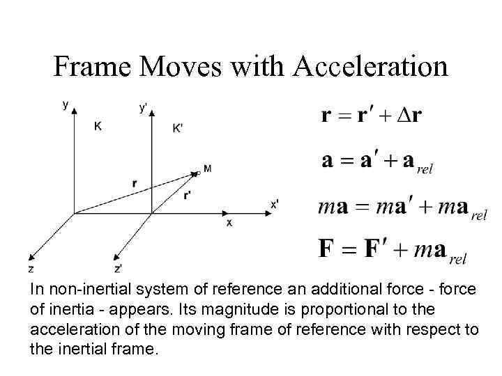
So, the effective net force on P1 in the frame of P2 is:
${\overrightarrow{F^{\prime }}}_{\text{net}}=m_1\vec{g}+(-m_1\vec{g})=\vec{0}$

Since the effective net force is zero, the acceleration observed in the non-inertial frame must also be zero:
${\overrightarrow{a^{\prime }}}_{1\text{ rel }2}=\frac{{\overrightarrow{F^{\prime }}}_{\text{net}}}{m_1}=\vec{0}$
This confirms our kinematic result and provides a deeper, more satisfying physical picture. The "magic" of the straight-line motion is explained by the perfect cancellation of the real force of gravity by the fictitious force arising from the observer's own accelerated motion.

A More Tangible Example: Pendulum in an Accelerating Car

Let's see how this force-based approach works in a different context.

This example shows how an object's equilibrium state (and thus its "trajectory" if it were oscillating) is altered in a non-inertial frame. The analysis is made simple by treating the fictitious force as just another force in the free-body diagram.

4. Beyond Linear Acceleration: A Glimpse into Rotating Frames

We have focused on linearly accelerating frames. You appreciate mathematical completeness, so it's important to acknowledge that this is a special case. The most general form of motion for a reference frame involves both linear acceleration and rotation.

When a frame rotates, the transformation equations become more complex, giving rise to additional, velocity-dependent fictitious forces. You may have heard of these: the Coriolis force and the centrifugal force. The full derivation is a beautiful exercise in vector calculus.

To give you a sense of this more general theory, the following video provides a rigorous, step-by-step derivation of the complete acceleration transformation for a frame that is both translating and rotating.

This derivation shows how the simple $\vec{a}=\vec{A}+\overrightarrow{a^{\prime }}$ relationship is just the beginning. The additional terms in a rotating frame are responsible for phenomena ranging from the circular motion of cyclones on Earth to the precession of a Foucault pendulum. We will not delve deeper into solving problems with these forces now, but having seen their origin is essential for a complete understanding of non-inertial frames. For a textual reference that also provides this derivation, you can consult the "Rotating Frames" section of the resource Non-inertial Frames, Translation and Rotating Coordinate ... (ID: LINK).

Conclusion

In this lesson, we moved from deriving transformation equations to actively applying them. By choosing a non-inertial frame wisely, we saw how a complex trajectory problem can be dramatically simplified.

Key Takeaways:

• The trajectory of an object as seen from a non-inertial frame can be found either kinematically, using $\overrightarrow{a^{\prime }}=\vec{a}-\vec{A}$, or dynamically, by adding the fictitious force ${\vec{F}}_{\text{fict}}=-m\vec{A}$ to the real forces. Both methods yield the same result.
• For any two objects moving under the same constant acceleration field (like gravity), their relative motion is uniform and linear.
• This principle allows us to solve advanced problems, such as finding the minimum separation between projectiles, by transforming them into simpler geometric exercises.
• Linearly accelerating frames are a special case. General non-inertial motion includes rotation, which introduces additional fictitious forces like the Coriolis and centrifugal forces.

Preview of the Next Lesson:
We have now derived the equations and seen how to apply them to analyze motion from either the inertial or non-inertial perspective. In the next lesson, we will focus on problem-solving strategy. We will solve problems conceptually from both an inertial and a linearly accelerating frame to demonstrate the equivalence of the kinematic description and to develop an intuition for when one approach is more advantageous than the other.