Bond Price Approximation: Duration & Convexity

Introduction

In our last two lessons, we developed the core tools for measuring interest rate risk: Modified Duration for a first-order (linear) approximation and Convexity for a second-order (curvature) measure. We saw that duration alone is insufficient for large yield changes because it ignores the curved nature of the price-yield relationship. Today, we will synthesize these concepts.

This lesson focuses on constructing a more robust model for predicting bond price changes. By combining duration and convexity, we will formulate the second-order Taylor expansion for the bond price function. This will provide a significantly more accurate estimate of a bond's price sensitivity, moving us closer to a professional-grade risk management tool.

From Linear to Quadratic Approximation

Before applying this to bonds, let's revisit the core mathematical idea. We are trying to approximate a complex, curved function with a simpler polynomial. A first-order (linear) approximation uses a tangent line. A second-order (quadratic) approximation uses a parabola that "hugs" the original curve much more closely.

Taylor Expansion Approximation of Loss Function — This graph illustrates the power of a second-order approximation. The actual function (blue curve) is poorly estimated by the linear approximation (red line) away from the point of tangency. The quadratic approximation (green curve), which incorporates curvature, provides a much better fit. This is precisely our goal: moving from the red line (duration) to the green line (duration + convexity).

To understand how these better-fitting polynomials are constructed, the following video provides an exceptionally clear, visual intuition.

Taylor series | Chapter 11, Essence of calculus

The video "Taylor series" from the 3Blue1Brown channel masterfully explains the logic behind building polynomial approximations.

Watch these segments to see how an approximation is built term by term: Introduction (from the start): This sets the stage for why we need to approximate functions with polynomials. Building a Quadratic Approximation (step-by-step): This is the most crucial part. Pay close attention to how the constants c_0, c_1, and c_2 are chosen to match the function's value, its first derivative (slope), and its second derivative (curvature) at a specific point. The General Formula (in full generality): This section presents the complete Taylor polynomial formula, which formalizes the process you just observed.

Formulating the Second-Order Price Approximation

The 3Blue1Brown video gives us the general recipe for a Taylor polynomial that approximates a function $f (x)$ around a point $a$ :
$f (x) \approx f (a) + f^{'} (a) (x - a) + \frac{f ^{''} ( a )}{2 !} (x - a)^{2}$

Now, let's translate this directly into the language of bond pricing.

Our function $f (x)$ is the bond's price, $P (y)$ .
Our variable $x$ is the yield, $y$ .
The point of approximation $a$ is the current yield, $y_{0}$ .
The change in yield, $(x - a)$ , is $Δ y = y - y_{0}$ .

Substituting these into the Taylor formula gives us the approximate new price, $P (y)$ :

$P (y) \approx P (y_{0}) + P^{'} (y_{0}) Δ y + \frac{P ^{''} ( y _{0} )}{2} (Δ y)^{2}$

where $P^{'} (y_{0})$ and $P^{''} (y_{0})$ are the first and second derivatives of the price function evaluated at the current yield.

From our previous lessons, we know the definitions of Dollar Duration and Dollar Convexity:

Dollar Duration = $- P^{'} (y_{0})$ (Note the negative sign)
Dollar Convexity = $P^{''} (y_{0})$

Substituting these into the approximation gives us the change in price in dollar terms:
$Δ P = P (y) - P (y_{0}) \approx (- Dollar Duration) \cdot Δ y + \frac{1}{2} Dollar Convexity \cdot (Δ y)^{2}$

This is a valid formula, but it's more common in practice to work with percentage price changes using Modified Duration and Convexity. To get there, we divide the entire equation by the initial price $P (y_{0})$ :

$\frac{Δ P}{P} \approx \frac{P ^{'} ( y _{0} )}{P ( y _{0} )} Δ y + \frac{1}{2} \frac{P ^{''} ( y _{0} )}{P ( y _{0} )} (Δ y)^{2}$

Recalling the definitions of Modified Duration and Convexity:

Modified Duration ( $D_{m o d}$ ) = $- \frac{1}{P} \frac{d P}{d y}$
Convexity ( $C$ ) = $\frac{1}{P} \frac{d ^{2} P}{d y ^{2}}$

We arrive at the final, canonical formula for the second-order approximation of the percentage change in bond price:

$\frac{Δ P}{P} \approx - D_{m o d} \cdot Δ y + \frac{1}{2} C \cdot (Δ y)^{2}$

This equation is the central outcome of this lesson. It shows that the estimated price change is the linear impact of duration plus a quadratic adjustment for convexity.

The following document from the University of Florida confirms this formulation.

Relative Impact of Duration and Convexity on Bond Price Changes

This paper by Brooks and Livingston formally presents the Taylor series expansion in the context of bond pricing.

Focus on Section I, "Taylor Series Expansion". Note how their equation (2) is precisely the formula we just derived, representing the percentage price change using the first and second derivative terms. This confirms our formulation is standard in finance literature.

The Full Picture: Formula and Visualization

The formula we derived beautifully captures the geometry of the price-yield curve.

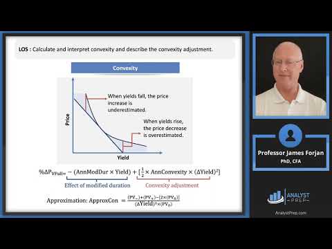
Bond Convexity and Price Approximation — This image provides a complete summary. The graph shows the actual price curve and the less accurate tangent line (duration). The formula at the bottom, `Approximate % change in full price`, is exactly what we derived: a linear term for duration and a quadratic adjustment for convexity.

Notice the convexity adjustment term, $\frac{1}{2} C \cdot (Δ y)^{2}$ . Since $C$ is positive for a standard bond and $(Δ y)^{2}$ is always non-negative, the convexity adjustment is always positive. This explains why the duration-only approximation consistently underestimates the bond's actual price, as seen in the graph. Convexity provides the "upward correction" to the linear estimate, improving accuracy whether yields rise or fall.

A Practical Example

Let's see this formula in action. The following video provides a clear, step-by-step example of how to use duration and convexity to estimate a bond's price change for a given yield shock.

Fixed Income: Duration plus convexity to approximate bond price change (FRM T4-38)

The video "Duration plus convexity to approximate bond price change" by Bionic Turtle is an excellent practical demonstration.

Watch these two key segments: Calculating the Percentage Change (applying the formula): The narrator calculates the price change using the percentage-based formula we derived. Observe how the total estimated change is the sum of the (symmetrical) duration effect and the (always positive) convexity adjustment. Notice how remarkably close the final approximation is to the actual repriced bond value. The Dollar Change Formulation (Tuckman's approach): This section shows an equivalent way to calculate the approximation in dollar terms, connecting directly to the concepts of dollar duration (the first derivative) and dollar convexity (the second derivative). This reinforces that both formulations are mathematically identical, just scaled differently.

Conclusion

In this lesson, we have successfully combined duration and convexity into a single, powerful model for estimating bond price changes. By grounding our work in the Taylor series expansion, we moved from separate first and second-order risk measures to an integrated second-order approximation.

Key Takeaways:

The second-order approximation for the percentage change in bond price is given by:
$\frac{Δ P}{P} \approx - D_{m o d} \cdot Δ y + \frac{1}{2} C \cdot (Δ y)^{2}$
This formula combines a linear estimate from Modified Duration with a quadratic correction from Convexity.
The convexity adjustment, $\frac{1}{2} C \cdot (Δ y)^{2}$ , is always positive for a standard bond, correcting for the systematic underestimation of the duration-only model.
This second-order model is substantially more accurate than the linear model, especially for larger changes in yield.

In our next lesson, we will put this knowledge into practice. You will implement the convexity calculation in Python and create a function to compare the price estimates from three models: the actual repriced bond, the first-order (duration) approximation, and the second-order (duration + convexity) approximation. This will allow us to visually and quantitatively assess the improvement in accuracy our new model provides.

Recommended resources