Welcome to the first lesson in your course on Categorical Data Analysis (CDA) and Generalized Linear Models (GLM).
This foundational lesson addresses a crucial first step in any data analysis project: understanding your data. We will focus on distinguishing between different types of data—specifically nominal, ordinal, and categorical data. You will also learn to identify the correct summary statistics and visualizations for each type.
Mastering this is essential because almost every statistical method you'll learn in this course, from a simple chi-square test to a complex logistic regression model, depends on correctly identifying the type of data you're working with. This knowledge forms the bedrock for everything that follows.
Let's begin.
1. The Landscape of Data: A Classification
At the highest level, data variables can be split into two main groups: categorical (qualitative) and numerical (quantitative).
- Categorical variables represent groupings or labels. Examples include gender, country of origin, or satisfaction level (e.g., "satisfied," "neutral," "dissatisfied").
- Numerical variables represent measurable quantities. Examples include height, temperature, or the number of clicks on a webpage.
This course will focus heavily on analyzing categorical data, but understanding the complete picture is vital. The flowchart below gives you a map of the main data types we'll discuss.
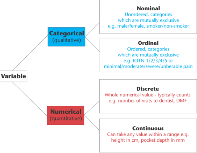
To get a formal introduction to these concepts, please watch the first part of the following video. It clearly defines the four main levels of measurement: nominal, ordinal, interval, and ratio.
This video from Prof. Patrick Meyer provides clear definitions of the four fundamental data types. It will help you build a solid vocabulary for the rest of the course.
Watch the segment from the beginning until 04:26. Pay close attention to the key characteristic of each data type: whether it has order, and whether the intervals between values are equal.
As you saw in the video, we can summarize the hierarchy of data as follows:
- Nominal: Purely categorical. Values are distinct labels with no inherent order.
- Examples: Eye color (blue, brown, green), political affiliation, type of car.
- Ordinal: Categorical with a meaningful order, but the intervals between the ranks are not necessarily equal or measurable.
- Examples: Education level (High School, Bachelor's, Master's, PhD), customer satisfaction (Very Unsatisfied, Neutral, Very Satisfied). The gap between "High School" and "Bachelor's" isn't the same as between "Master's" and "PhD".
- Interval: Numerical data that is ordered and has equal intervals between values, but lacks a "true zero." A value of zero does not mean the absence of the quantity.
- Examples: Temperature in Celsius or Fahrenheit (0°C doesn't mean no heat), IQ scores. You can't say 20°C is "twice as hot" as 10°C.
- Ratio: The most informative level. It is ordered, has equal intervals, and a "true zero," which represents the complete absence of the attribute.
- Examples: Height, weight, age, income in dollars. A weight of 0 kg means no weight. You can say someone who is 2 meters tall is twice as tall as someone who is 1 meter tall.
For the purposes of this course, we will primarily group these into three buckets: Nominal, Ordinal, and Numerical (which combines Interval and Ratio).
2. A Closer Look at Categorical Data
Let's now focus on nominal and ordinal data, as they are the stars of categorical data analysis. The infographic below provides a side-by-side comparison.

To deepen your functional understanding, let's explore these types with more examples. The following reading and video provide concise definitions and practical illustrations. A special type of nominal data, binary data, consists of only two categories (e.g., Yes/No, Pass/Fail). It's extremely common in data science.
1 Collecting and Summarizing Data – STAT 500 - Statistics Online
This resource from Penn State's STAT 500 course offers clear, textbook-style definitions of qualitative (categorical) data, including the important distinction of binary data.
Please read section 1.2, titled 'Classifying Data.' Focus on the definitions and examples for Qualitative (Categorical) data, including Binary, Ordinal, and Nominal types.
Now, watch the following video. It offers a slightly different perspective and a helpful applied example at the end, which reinforces the concepts.
Types of Data: Nominal, Ordinal, Interval/Ratio - Statistics Help
This video from Dr Nic's Maths and Stats provides another look at nominal and ordinal data, with a useful example of how these data types appear in a customer survey.
Please watch the sections covering nominal data (01:08 - 01:53), ordinal data (01:53 - 02:47), and the customer survey example (04:00 - 06:15). Notice the discussion about the appropriateness of calculating a mean for ordinal data—this is a key point for practical application.
Functional Understanding Check
A crucial insight for any data scientist is that the way you collect data determines its type.
Consider the "Exploratory Data Analysis" video (LINK) you watched earlier. It gave an excellent example where a survey asked about the number of books in a home, but provided these response options: '0-10', '11-50', '51-100', '101+'.
Question: What data type is this variable as collected by the survey, and why? How would the data type change if the survey simply asked respondents to enter the exact number of books they own?
Answer
The variable, as collected with response options like '0-10', is ordinal.
- Why? The categories have a clear order (more books are in '11-50' than '0-10'), but the intervals are unequal. The range of the first category is 11 books, while the second is 40. Because the distances aren't uniform, it cannot be treated as numerical (interval/ratio).
If the survey asked for the exact number of books, the data would be ratio (and also discrete numerical).
- Why? The values would be ordered counts (1, 2, 3...), the interval between each value is uniform (the difference between 5 and 6 books is the same as between 99 and 100), and there is a true zero (0 books means no books).
3. How to Summarize Categorical Data
Now that you can identify nominal and ordinal data, how do you describe a dataset composed of them? The choice of summary measure is dictated by the data's properties.
We use:
- Measures of Central Tendency: To find a "typical" value (e.g., mode, median).
- Measures of Distribution/Variability: To describe how the data is spread across categories (e.g., frequencies, range).
- Visualizations: To see the distribution at a glance (e.g., bar charts, pie charts).
The following table summarizes which measures are appropriate for each categorical data type.
| Data Type | Central Tendency | Distribution/Variability | Visualization |
|---|---|---|---|
| Nominal | Mode | Frequencies, Proportions/Percentages | Bar chart, Pie chart |
| Ordinal | Median, Mode | Frequencies, Proportions, Range, Inter-quartile Range (IQR) | Bar chart (ordered) |
Why these measures?
- Mode: The most frequent category. It works for both nominal and ordinal data because it doesn't require any sense of order.
- Frequencies/Proportions: Simple counts of how many observations fall into each category. This is the most fundamental way to summarize any categorical variable.
- Median: The middle value after the data has been ordered. This is why it's suitable for ordinal data but meaningless for nominal data (you can't find the "middle" eye color).
- Mean (Average): You should generally avoid calculating the mean for categorical data. What is the average of "blue," "green," and "brown"? The question makes no sense. While some researchers compute means for ordinal data (like 1-5 satisfaction scores), this assumes the intervals are equal, which is often not true. This is a common but questionable practice.
- Range & IQR: These measures of spread rely on ordering the data from minimum to maximum. Therefore, they are applicable to ordinal data but not nominal data.
To solidify your understanding of these summary measures, please review the following resource.
Week 2: Describing Categorical Data
This webpage from a University of Edinburgh course provides concise definitions for the key summary measures used with categorical data. It clearly links each measure to the appropriate data type.
Read through the slides that define and explain the key summary measures. You can navigate using the numbers at the bottom (e.g., 15/30). Start at slide 15 to see the mapping of measures to data types. Review the definitions of Mode (slide 17), Median (slide 20), Range (slide 24), and Inter-quartile range (IQR) (slide 25). Don't worry about the R code examples; focus on the concepts.
Conclusion
In this lesson, we established the critical first step of any data analysis workflow: classifying variables.
Key Takeaways:
- Data can be broadly classified as categorical (labels) or numerical (quantities).
- Categorical data is further divided into:
- Nominal data: Unordered categories (e.g.,
Male,Female). - Ordinal data: Ordered categories where the distance between them is not uniform (e.g.,
Low,Medium,High).
- Nominal data: Unordered categories (e.g.,
- The type of data determines the appropriate summary measures:
- For nominal data, use frequencies, proportions, and the mode. Visualize with bar or pie charts.
- For ordinal data, you can also use the median, range, and inter-quartile range (IQR) because the data has a meaningful order.
Understanding these distinctions is not just academic; it has profound practical implications for choosing the right statistical tests and models, which is the entire focus of this course.
Preview of the Next Lesson:
Now that you can describe a single categorical variable, we will move on to exploring the relationship between two categorical variables. We will learn how to construct and interpret a contingency table, a fundamental tool for categorical data analysis.