Poisson Regression: Modeling Counts and Interpreting the Log Link

1. Why is Count Data Different?

Before we introduce a new model, it's important to understand why our existing tools, like ordinary linear regression, are often inappropriate for count data.

Count data has several distinct characteristics:

• Non-negative integers: Counts can only be 0, 1, 2, ... and never negative or fractional.
• Skewed distribution: The data is often right-skewed, with most observations having low counts and a few having very high counts.
• Variance related to the mean: Unlike the assumption of constant variance (homoscedasticity) in linear regression, with count data, the variance tends to increase as the mean count increases.

Applying a simple linear model to count data can lead to several problems, including nonsensical predictions.

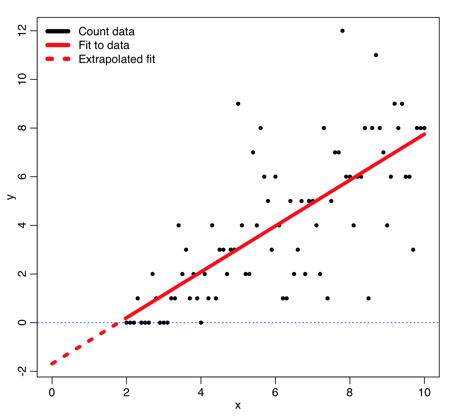
The following video provides a clear, quick summary of these issues.

To address these issues, we need a model that is specifically designed for the properties of count data. This brings us to Poisson regression.

2. The Poisson Regression Model: A GLM Approach

As you'll recall from our discussions on logistic regression, a Generalized Linear Model (GLM) provides a flexible framework for modeling different types of response variables. Poisson regression is a GLM tailored for count data.

To understand its structure, let's review the three core components of any GLM. The following reading provides a great refresher and applies it directly to count data models.

As you just read, the three components for a Poisson regression model are:

1. Random/Stochastic Component: The response variable $Y_i$ (the count) is assumed to follow a Poisson distribution. A key property of the Poisson distribution is that its mean and variance are equal. We denote the mean (and variance) as $\lambda$.

   $$Y_i\sim \text{Poisson}({\lambda }_i)$$

   This directly addresses the issue that variance often increases with the mean in count data.

2. Systematic Component: This is the linear predictor, which is a linear combination of the explanatory variables ($x$). It has the same form as in linear regression.

   $${\eta }_i={\beta }_0+{\beta }_1{x}_{i1}+{\beta }_2{x}_{i2}+\cdots +{\beta }_p{x}_{ip}$$

3. Link Function: This function, $g()$, connects the mean of the response, ${\lambda }_i$, to the linear predictor, ${\eta }_i$. For Poisson regression, the standard and canonical link function is the natural logarithm (log) link.

   $$g({\lambda }_i)=\log ({\lambda }_i)$$

3. Formulating the Model and the Role of the Log Link

Putting these three components together, we get the formal Poisson regression model:

This equation states that the log of the mean count is a linear function of the predictors. This is the "formulation" of the model. Now, let's explore why this log link is so important.

What does the log link do?

1. Ensures Positive Predictions: By modeling the log of the mean, we ensure that the predicted mean count itself is always positive. If we rearrange the equation, we get:

   $${\lambda }_i=e^{({\beta }_0+{\beta }_1{x}_{i1}+\cdots +{\beta }_p{x}_{ip})}$$

   Since the exponential function $e^x$ always returns a positive value, our model's predicted mean count, ${\hat{\lambda }}_i$, can never be negative. This elegantly solves one of the major problems of using linear regression.

2. Linearizes the Relationship: The log link transforms a non-linear, multiplicative relationship on the original "response scale" into a linear, additive relationship on the "link scale."

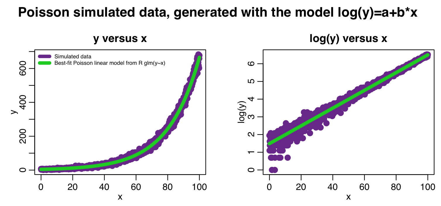
The following reading provides a concise summary of the Poisson regression model, its assumptions, and reinforces the role of the log link.

4. Interpreting Coefficients with a Log Link

Understanding the log link is critical for correctly interpreting the model's coefficients (${\beta }_j$).

In a linear model, ${\beta }_j$ is the change in the mean response for a one-unit change in $x_j$. In Poisson regression, ${\beta }_j$ is the change in the log of the mean response for a one-unit change in $x_j$. This "log-scale" interpretation isn't very intuitive.

To get a more practical interpretation, we need to back-transform from the log scale. Let's see how this works for a simple model with one predictor, $x$:

1. For a value of $x$, the log-mean is: $\log ({\lambda }_x)={\beta }_0+{\beta }_{1}x$
2. For a value of $x+1$, the log-mean is: $\log ({\lambda }_{x+1})={\beta }_0+{\beta }_1(x+1)$

Subtracting the first equation from the second gives us:

Using the properties of logarithms ($\log (a)-\log (b)=\log (a/b)$), we get:

Finally, by exponentiating both sides, we isolate the ratio of the means:

This quantity, $e^{{\beta }_1}$, is called the Rate Ratio (RR) or Incidence Rate Ratio (IRR).

This leads to our key interpretation:

For a one-unit increase in $x$, the mean count $\lambda$ is multiplied by a factor of $e^{{\beta }_1}$.

For example, if ${\beta }_1=0.2$, then $e^{0.2}\approx 1.22$. This means a one-unit increase in $x$ is associated with a 22% increase in the mean count. If ${\beta }_1=-0.1$, then $e^{-0.1}\approx 0.90$, meaning a one-unit increase in $x$ is associated with a 10% decrease in the mean count.

The following resources walk through this interpretation with clear examples.

Conclusion

In this lesson, we have laid the groundwork for analyzing count data. We established why linear regression is unsuitable and how Poisson regression provides a robust, theoretically sound alternative within the GLM framework.

Key Takeaways:

• Count data is non-negative, integer-valued, and often exhibits a mean-variance relationship that violates the assumptions of linear regression.
• Poisson regression is a GLM that assumes a Poisson distribution for the response variable (the random component).
• It uses a log link function to connect the mean of the count ($\lambda$) to a linear predictor ($\eta$).
• The model is formulated as: $\log (\lambda )=\mathbf{X}\mathbf{\beta }$.
• The log link serves two critical purposes: it ensures all predicted mean counts are positive and it linearizes the model's structure.
• A coefficient ${\beta }_j$ is interpreted by exponentiating it: $e^{{\beta }_j}$ is the Rate Ratio, representing the multiplicative change in the mean count for a one-unit increase in the predictor $x_j$.

Preview of the Next Lesson:
Now that you understand the structure of the model and the principle behind interpreting its coefficients, we will move on to a more hands-on application. In the next lesson, we will focus on fitting a Poisson regression model to data and practicing the conversion of coefficients into interpretable rate ratios with confidence intervals.