Log-Linear Models for Multi-Way Tables

1. The Goal: Uncovering the Association Structure

When we have three or more categorical variables, simply asking "are they related?" is not enough. The relationships can be complex. For example, two variables might only be related through a third, or their relationship might change depending on the level of the third variable. A "log-linear analysis" is the process of finding the simplest model that accurately describes this pattern of dependence and independence.

Let's visualize the possibilities for three variables: A, B, and C.

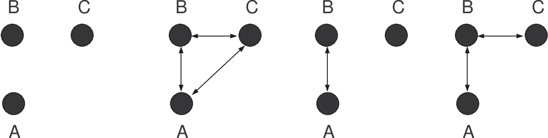
The main patterns we test for are:

1. Complete Independence: (Top-left graph) A, B, and C are all unrelated. The log-linear model is A + B + C.
2. Conditional Independence: (Bottom-right graph) A and C are only related through their shared connection with B. If you hold B constant, A and C become independent. The model is AB + BC.
3. Homogeneous Association: (Not perfectly depicted, but related to the bottom-left/right) All pairs of variables are associated, but the strength of association between any two (e.g., A and B) is the same across all levels of the third variable (C). There is no three-way interaction. The model is AB + AC + BC.
4. Saturated Model: (Top-right graph) The model includes a three-way interaction (A*B*C). This means the relationship between two variables changes depending on the level of the third.

Our strategy is to start with the simplest model and add complexity, stopping when we find a model that fits the data well. We assess "fit" using the model's deviance.

2. A Case Study: Educational Aspirations

Let's apply this strategy to a classic dataset.

Our goal is to understand the association structure between Status (S), Encouragement (E), and Plans (P). Are they all independent? Do they interact in pairs? Or is there a complex three-way interaction?

3. The Analysis: A Hierarchical Approach

We will now fit a series of hierarchical log-linear models. We'll start simple and add complexity, checking the deviance at each step. Remember from our previous lessons, the deviance is a goodness-of-fit statistic. A large, significant deviance means the model fits poorly, while a small, non-significant deviance means the model fits the data well.

The document you just read provides a perfect summary of this process in its Table 5.3.

Let's interpret this table step-by-step.

Step 1: Test for Complete Independence

The simplest hypothesis is that S, E, and P are all mutually independent. This corresponds to the model S + E + P.

• From Table 5.3: The deviance is 2714.0 with 10 d.f.
• Interpretation: This deviance is extremely large and would have a p-value close to zero. The model is a very poor fit.
• Conclusion: We strongly reject the hypothesis of complete independence. The variables are associated.

Step 2: Test Models with One Interaction

Let's see if a model where two variables are associated, but jointly independent of the third, is a good fit. An example is SE + P, which tests if parental encouragement and socio-economic status are related, but jointly independent of college plans.

• From Table 5.3: The models SE + P, SP + E, and S + EP all have very large, significant deviances.
• Conclusion: These simpler structures are not sufficient. The data shows a more complex pattern of associations.

Step 3: Test Models with Two Interactions (Conditional Independence)

Now we test for conditional independence. For example, the model SE + SP proposes that parental encouragement (E) and college plans (P) are independent conditional on a student's socio-economic status (S).

• From Table 5.3: The models SE + SP, SE + EP, and SP + EP still have large and highly significant deviances (e.g., SE + SP has a deviance of 1083.8 with 4 d.f.).
• Conclusion: We reject the hypotheses of conditional independence. For example, the relationship between parental encouragement and college plans is significant even after accounting for socio-economic status.

Step 4: Test the Homogeneous Association Model

This is the most complex model short of the saturated model. The model SE + SP + EP includes all possible two-way interactions. It hypothesizes that while all pairs of variables are associated, the strength of the association between any two variables is the same across all levels of the third.

• From Table 5.3: The deviance is 1.575 with 3 d.f.
• Interpretation: This deviance is very small. The corresponding p-value would be large (p > 0.05), indicating that the model's expected counts are not significantly different from the observed counts.
• Conclusion: This model fits the data very well!

We have found our answer. The association structure is one of homogeneous association.

4. Interpreting the Final Model

What does "homogeneous association" mean in this context?

The key takeaway from the reading is this:

The model SE + SP + EP tells us that the association between any two variables is consistent across the levels of the third. Specifically, the association between parental encouragement (E) and college plans (P) is the same in all socio-economic strata (S).

The author even calculates the odds ratio between encouragement and plans, finding it to be 14.6 for every single social class. This is a powerful and specific finding. A simple chi-square test on the whole table wouldn't have given us this nuanced insight.

5. Practical Application with Code

You've seen the logic, but how would you run this yourself? As we learned, you would use a GLM function for Poisson regression.

As the examples show, you would fit the competing models (e.g., the homogeneous association model and the saturated model) and compare their deviances (Likelihood Ratio Chi Square in the output) to test the significance of the highest-order interaction term. A non-significant result for that term, as seen in the sample write-up (G2(1) = .03, p = .86), justifies using the simpler homogeneous association model.

Conclusion

This lesson brought together the theory of log-linear models and the practice of Poisson regression to perform a complete analysis of a multi-way contingency table.

Key Takeaways:

• Log-linear analysis allows us to move beyond a simple "is there a relationship?" to describe the specific association structure in multi-way tables.
• The standard approach is to fit a hierarchy of models, from simplest (complete independence) to most complex (saturated).
• We select the most parsimonious model (the simplest one) that provides a good fit to the data, as judged by a non-significant deviance (Likelihood Ratio Chi-Square).
• The chosen model provides an interpretable story. For our case study, the model of homogeneous association (SE + SP + EP) revealed that the odds of planning for college are strongly associated with parental encouragement, and this effect is consistent across all socio-economic groups.

Course Wrap-up

Congratulations! You have reached the end of our course on Categorical Data Analysis and Generalized Linear Models.

We began by exploring the fundamentals of categorical data with contingency tables and chi-square tests. We then transitioned into a modeling framework, starting with Binary Logistic Regression for two-category outcomes, expanding to Multinomial and Ordinal Logistic Regression for more complex outcomes, and tackling specialized cases like matched data with Conditional Logistic Regression.

Finally, we moved to count data with Poisson Regression and saw how it provides a powerful engine for fitting Log-Linear Models, unifying the entire field of contingency table analysis within the flexible GLM framework.

You have developed a robust, practical, and functional understanding of how to model non-normal dependent variables—a critical skill set for modern data science. I hope this structured journey has equipped you with the confidence to apply these methods in your master's program and beyond. Well done