Conditional Likelihood in Logistic Regression

The Problem: Too Many Parameters

Let's quickly restate the core problem. When we have matched data, like case-control pairs, each pair (or stratum) has its own unique baseline risk. In a logistic regression model, we represent this with a stratum-specific intercept, ${\alpha }_k$:

The ${\alpha }_k$ terms are called nuisance parameters. They are necessary to correctly specify the model and account for the matching, but we aren't interested in their specific values. The problem is that in a 1-to-1 matched study, the number of ${\alpha }_k$ parameters is half the sample size! As we add more pairs, we add more nuisance parameters. This is the Incidental Parameters Problem, and it leads to biased estimates of $\beta$, the coefficient we actually care about.

The following video provides an excellent explanation of this problem and why traditional methods fail.

The Solution: Changing the Question with Conditioning

Since trying to estimate the ${\alpha }_k$ parameters fails, conditional logistic regression takes a different, more elegant approach. It changes the question being asked.

Instead of modeling the absolute probability of being a case, CLR models a conditional probability. For a 1-to-1 matched pair, the question becomes:

Given that one person in this pair is the case and the other is the control, what is the probability that the individual with exposure profile ${\mathbf{x}}_{\text{case}}$ is, in fact, the case?

This "given" part is the act of conditioning. We are building our analysis on the subset of information where we know there's exactly one positive outcome in the pair. This condition contains all the necessary information about the nuisance parameter ${\alpha }_k$. By making it a condition of our analysis, we effectively remove ${\alpha }_k$ from the equation that needs to be solved.

The following reading explains exactly how this is done.

The Magic of Cancellation

As the reading explained, the key is the construction of the conditional likelihood. Let's walk through the logic without getting lost in complex derivations.

Consider a single matched pair $k$, consisting of the actual case (subject 1) and control (subject 2).

• The case has exposure vector ${\mathbf{x}}_{1k}$.
• The control has exposure vector ${\mathbf{x}}_{0k}$.

The conditional probability we want is:

The denominator is the sum of probabilities of the two ways this could happen: (Subject 1 is case, Subject 2 is control) OR (Subject 1 is control, Subject 2 is case).

When we write this out using the logistic regression formula, the ${\alpha }_k$ term appears in every part of the expression. Let's see the crucial step. The probability becomes:

The standard logistic probability is $\pi (\mathbf{x})=\frac{e^{{\alpha }_k+{\beta }^{\prime }\mathbf{x}}}{1+e^{{\alpha }_k+{\beta }^{\prime }\mathbf{x}}}$. After substituting this into the expression above and simplifying, we arrive at the conditional likelihood contribution for pair $k$:

Now, notice that we can factor out $e^{{\alpha }_k}$ from the denominator:

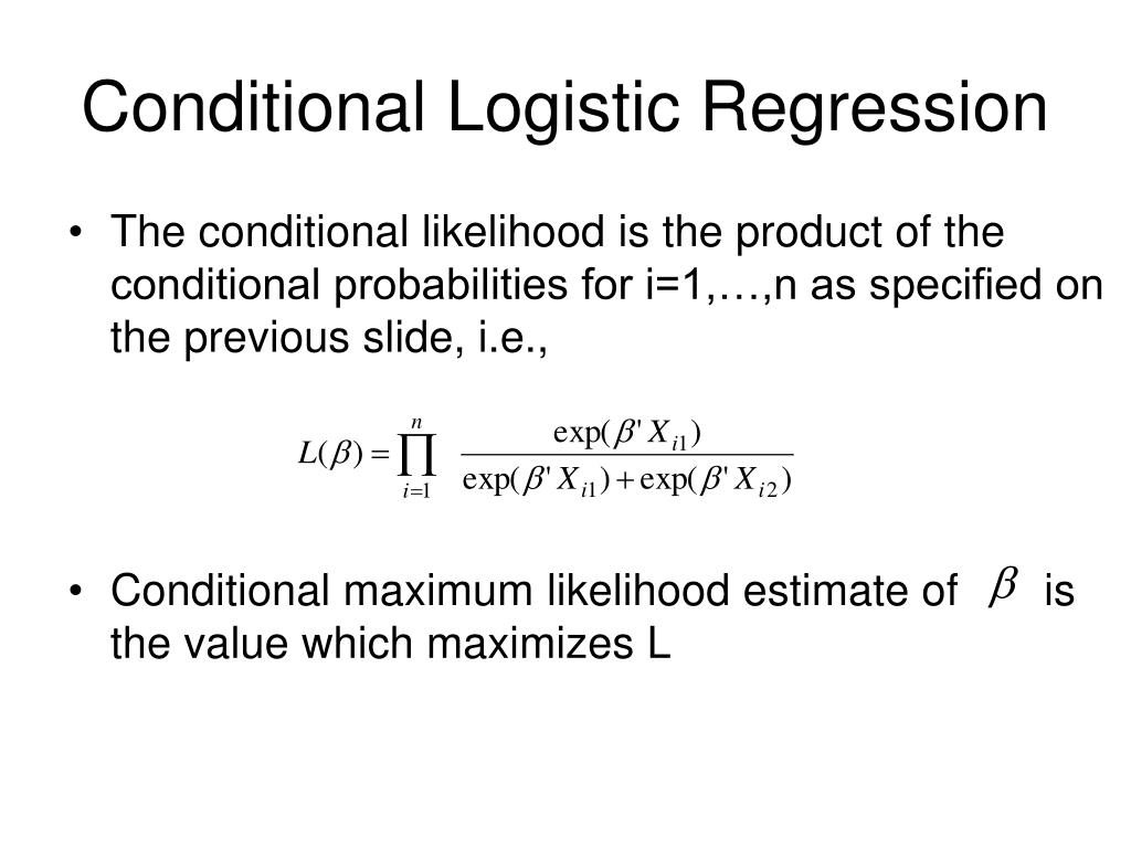
The $e^{{\alpha }_k}$ term in the numerator and denominator cancels out, leaving us with a beautiful, clean expression that depends only on $\beta$ and the observed exposure data:

This is the conditional likelihood for one pair. The nuisance parameter ${\alpha }_k$ is gone! We have successfully "conditioned it out" of the problem. This is the core mechanism you need to understand.

This slide provides a concise visual summary of the final likelihood function.

What this Means Functionally

Eliminating the nuisance parameter isn't just a mathematical trick; it has important practical consequences.

1. Focus on Relative Probabilities: The model no longer estimates the absolute risk for any individual. It can't, because the baseline risk (${\alpha }_k$) has been removed. Instead, it models the relative probability (or odds) that a person with one set of exposures is the case compared to another person within the same matched set. The hockey team example from the video you watched earlier is a great analogy for this.

2. Only Discordant Pairs Contribute: As we touched on in the last lesson, this formulation means that if a case and a control have the exact same exposure profile (${\mathbf{x}}_{1k}={\mathbf{x}}_{0k}$), their contribution to the likelihood is:
   $L_k(\beta )=\frac{e^{{\beta }^{\prime }\mathbf{x}}}{e^{{\beta }^{\prime }\mathbf{x}}+e^{{\beta }^{\prime }\mathbf{x}}}=\frac{1}{2}$
   This term is a constant and provides no information for estimating $\beta$. This confirms the intuition that only discordant pairs, where the exposures differ, can tell us about the exposure's effect.

3. Cannot Estimate Effects of Matched Variables: A direct consequence of this is that you cannot estimate the effect of any variable that you used for matching. If you match cases and controls on age, then age is constant within every pair. Just like with concordant exposures, it will cancel out and you cannot estimate its coefficient (${\beta }_{\text{age}}$).

Conclusion

Today we dove into the core mechanism of conditional logistic regression. You saw that it's not magic, but a clever statistical reframing of the research question.

Key Takeaways:

• CLR tackles the Incidental Parameters Problem by avoiding the estimation of nuisance parameters (${\alpha }_k$) altogether.
• It achieves this by constructing a conditional likelihood, which models the probability of the observed data given that a certain number of cases occurred within a matched set.
• In the process of deriving this conditional likelihood, the stratum-specific intercept term (${\alpha }_k$) appears in both the numerator and denominator, allowing it to be mathematically cancelled out.
• The resulting likelihood function depends only on the parameters of interest ($\beta$), which can then be estimated without bias from the nuisance parameters.
• This means the model focuses on relative, not absolute, probabilities and can only use information from pairs where the exposures differ (discordant pairs).

Preview of the Next Lesson:

Now that you have a solid conceptual and functional understanding of how CLR works, our next step is to put it into practice. In the next lesson, we will fit a conditional logistic regression model to a matched case-control dataset, interpret the resulting coefficients, and discuss how the output reflects the principles we've learned today.