Introduction
Welcome to our next lesson! In the last two sessions, we've built a solid foundation for analyzing paired categorical data measured at two points in time. You learned to use the McNemar test for binary outcomes (like "success/failure") and the Stuart-Maxwell test for outcomes with more than two categories (like "low/medium/high").
This naturally leads to a new question: What if we measure a binary outcome on the same subjects at three or more points in time? For instance, imagine a panel of voters is asked the same "yes/no" question before a debate, right after the debate, and one week later. The McNemar test can't handle this, as it's limited to two groups.
This lesson introduces the solution: the Cochran Q test. Our goal is to understand and apply this test, which is specifically designed to compare proportions for a binary variable across three or more related groups. You'll learn its purpose, how it extends the logic of the McNemar test, and how to interpret its results, including the crucial follow-up steps.
1. Positioning the Cochran Q Test
Before diving into the mechanics, it's essential to understand where the Cochran Q test fits within the landscape of statistical methods. It's a non-parametric test, meaning it doesn't assume the data follows a specific distribution like the normal distribution.
To clarify its role, let's compare it to some other tests you've encountered or will encounter soon.
Cochran's Q Test in SPSS - Performing, Reported, Explained
This article, 'Cochran's Q Test in SPSS', gives an excellent conceptual overview and clearly distinguishes the test from its common alternatives. This will help you build a mental map of when to use which tool.
Please read the first five sections, from 'Introduction' through 'When to use: Friedman Test, Cochran’s Q Test, Kendall’s W'. Focus on how the article defines Cochran's Q and differentiates it from McNemar's Test and Repeated Measures ANOVA.
From your reading, let's summarize the key distinctions:
| Test | When to Use It | Example |
|---|---|---|
| McNemar Test | 2 related groups, binary outcome. | Comparing the proportion of patients responding to a drug before vs. after treatment. |
| Cochran Q Test | 3 or more related groups, binary outcome. | Comparing the proportion of students passing a test at three different times in a semester. |
| Repeated Measures ANOVA | 3 or more related groups, continuous outcome. | Measuring the same person's blood pressure at three different times. |
| Friedman Test | 3 or more related groups, ordinal (ranked) outcome. | Having three wine experts rank the same four wines from best to worst. |
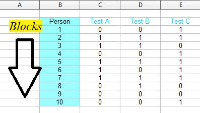
As you can see, the Cochran Q test is a direct generalization of the McNemar test. It fills the specific need for analyzing repeated binary measurements.
2. Hypotheses and Assumptions
Like any statistical test, Cochran's Q has a formal structure. Understanding its hypotheses and assumptions is key to using it correctly.
Cochran's Q Test in SPSS - Performing, Reported, Explained
The same article from SPSS Analysis also provides a very clear and concise summary of the test's assumptions and hypotheses.
Now, please read the sections 'The Assumptions of the Cochran’s Q Test' and 'The Hypothesis of the Cochran’s Q Test'.
Let's break these down:
Assumptions:
- Related Samples: The measurements are taken on the same subjects or matched subjects (e.g., the same person is tested three times).
- Binary Outcome: The variable of interest has only two possible outcomes (e.g., success/failure, yes/no, present/absent), typically coded as 1 and 0.
- Three or More Groups: There are at least three conditions or time points being compared.
Hypotheses:
- Null Hypothesis (): The proportions of "successes" (or the outcome coded as 1) are equal across all groups/conditions. For example, .
- Alternative Hypothesis (): The proportion of "successes" is not equal across all groups. At least one group's proportion is different from the others.
Rejecting the null hypothesis means we have evidence that the likelihood of the outcome changes across the conditions.
3. Application and Interpretation
Let's walk through a practical example to see how the test is applied and what the results tell us. We'll use an excellent guide from the "Real Statistics Using Excel" website.
Cochran's Q Test - Real Statistics Using Excel
This resource provides a step-by-step example of calculating and interpreting the Cochran Q test, which is perfect for understanding its functional application.
Please read the sections 'Using Raw Data' and review the text leading up to the 'Follow-up Testing' section. Pay attention to Example 1, the data in Figure 1, the calculated Q statistic in Figure 2, and the final interpretation of the p-value.
The Example: Worker Energy Levels
In this study, 20 workers are classified as "energetic" (1) or "tired" (0) on a Monday, Wednesday, and Friday.
- Null Hypothesis (): The proportion of energetic workers is the same on Monday, Wednesday, and Friday.
- Alternative Hypothesis (): The proportion of energetic workers differs on at least one of those days.
The Q Statistic
The resource shows the formula for the test statistic, . You don't need to memorize it, but it's useful to understand the intuition. The statistic essentially compares the variability in outcomes between the days (the column totals) to the variability within the workers (the row totals). A large value suggests that the differences between the days are greater than what you'd expect from random chance alone.
The calculated statistic follows a chi-squared distribution with degrees of freedom, where k is the number of groups (in this case, 3 days, so degrees of freedom).
The Result
From the analysis in the resource:
- p-value = 0.035
Since the p-value (0.035) is less than the conventional significance level of 0.05, we reject the null hypothesis. Our conclusion is that there is a statistically significant difference in the proportion of energetic workers across the three days.
4. Post-Hoc Analysis: Finding the Specific Differences
The Cochran Q test is an omnibus test. This means it tells you that a difference exists somewhere among the groups, but it doesn't tell you which specific groups are different. Did the proportion of energetic workers change from Monday to Wednesday? Or from Monday to Friday?
To find out, we must perform post-hoc tests.
Cochran's Q Test - Real Statistics Using Excel
Now, let's look at the crucial next step. The 'Real Statistics' resource explains how to conduct follow-up tests correctly.
Please read the section 'Follow-up Testing'. Focus on two key ideas: which test is used for the pairwise comparisons, and what the 'Bonferroni correction' is for.
Here's the procedure:
-
Conduct Pairwise Tests: We compare each pair of groups using the McNemar test. (As the resource notes, a Cochran Q test with only two groups is mathematically equivalent to a McNemar test). For our example, we would run three separate tests:
- Monday vs. Wednesday
- Monday vs. Friday
- Wednesday vs. Friday
-
Correct for Multiple Comparisons: Every time you run a hypothesis test, there's a chance of a false positive (a Type I error). When you run multiple tests, this chance accumulates. To control for this, we must adjust our significance level. The Bonferroni correction is a simple and common way to do this:
- New significance level () = Original significance level () / Number of comparisons
- In our case: .
-
Interpret the Corrected Results: We now compare the p-value of each individual McNemar test to our new, stricter significance level of 0.0167.
- The resource shows that none of the pairwise p-values (0.052, 0.021, 0.739) are less than 0.0167.
This leads to a nuanced but very important conclusion: "There is a significant difference (...) between the percentage of workers who are energetic on Monday (30%), Wednesday (65%), and Friday (70%), but none of the pairwise comparisons is significant [after correction]."
This might seem contradictory, but it means that while the overall pattern of change is statistically significant, no single pairwise jump is large enough to clear the higher bar set by the Bonferroni correction. The difference between Monday and Friday (p=0.021) was the closest to being significant.
Conclusion
In this lesson, you have added another essential tool for analyzing paired data to your toolkit. You've seen how the Cochran Q test extends the McNemar test to handle situations with more than two repeated measurements of a binary outcome.
Key Takeaways:
- Cochran's Q test is used to compare proportions for a binary outcome across three or more related groups.
- It is a non-parametric generalization of the McNemar test.
- The null hypothesis () is that the proportions are equal across all groups.
- The test is omnibus; a significant result indicates a difference exists somewhere, but does not specify where.
- Post-hoc tests (e.g., pairwise McNemar tests) with a correction for multiple comparisons (e.g., Bonferroni) are required to identify which specific groups differ.
Preview of the Next Lesson:
So far in this module, we have focused exclusively on test-based approaches like the McNemar, Stuart-Maxwell, and Cochran Q tests. These are powerful for answering the question, "Is there a significant difference?". However, they have limitations, particularly in their ability to account for other explanatory variables (covariates).
In the next lesson, we will pivot to a more flexible and powerful framework. We will contrast these test-based methods with a model-based approach, introducing the core ideas behind Conditional Logistic Regression. This will provide a crucial bridge to the second major topic in this course: Generalized Linear Models (GLMs).