Modeling Strategies for Violating Proportional Odds

The Fork in the Road: What to Do When the Assumption is Violated

When a Brant test fails, you have two main choices:

1. Abandon the ordering: You can switch to a model that treats the outcome variable as nominal (unordered).
2. Use a more flexible ordinal model: You can use a model that still acknowledges the outcome's order but doesn't impose the strict proportional odds assumption on all predictors.

Let's explore each of these paths.

Path 1: Multinomial Logistic Regression

The most straightforward alternative is to revert to a multinomial logistic regression model. As you may recall, this model is designed for nominal outcomes with more than two categories.

How it works:

• It chooses one outcome category as a reference (or baseline).
• It then builds $J-1$ separate logistic regression models, where $J$ is the number of categories. Each model estimates the odds of being in one specific category versus the reference category.
• This means you get $J-1$ sets of coefficients and odds ratios to interpret, one for each non-reference category.

The key trade-off here is between parsimony and precision. The following video explains this beautifully.

Summary of Multinomial Regression as an Alternative:

• Pro: It's a "safe" choice. It makes fewer assumptions and will always give you more precise estimates because it's not constrained by the proportional odds assumption.
• Con: It's not parsimonious. You lose the simple, single-odds-ratio interpretation of the ordinal model. More importantly, you discard the valuable information that your outcome categories have a natural order, which can lead to a loss of statistical power.

Because of this, while the multinomial model is a valid fallback, analysts often first explore more flexible ordinal models.

Path 2: More Flexible Ordinal Models

Instead of abandoning the ordinal nature of your data, you can use models that relax the proportional odds assumption. There are several such models, but we will focus on the most powerful and common family: Generalized Ordered Logit Models.

The lecture slides below provide a concise overview of the options available when you reject the proportional odds assumption. Notice that "Partial proportional odds" is a key strategy.

The Generalized Ordered Logit (Gologit) Model

The Gologit model is a more general form of the ordered logit model. Instead of estimating one set of coefficients ($\beta$) that applies across all cumulative splits, it estimates a separate set of coefficients (${\beta }_j$) for each split.

This is very flexible, but it results in a model that is just as complex as a multinomial model. Its real power comes from a special case: the Partial Proportional Odds (PPO) model.

The Partial Proportional Odds (PPO) Model

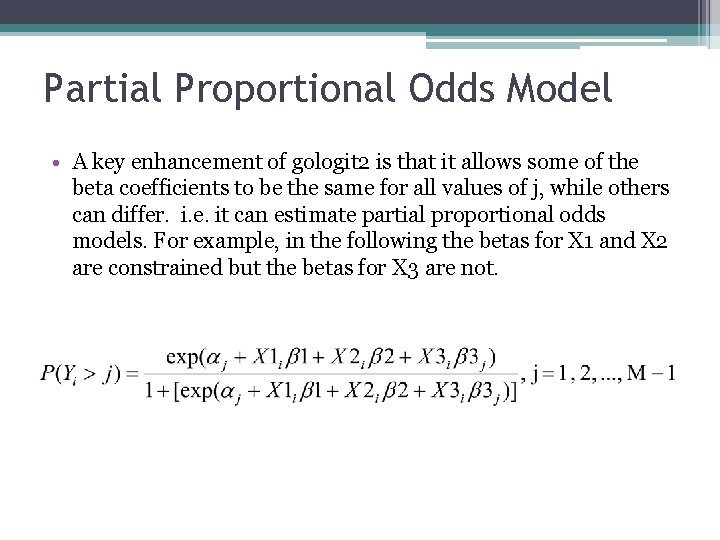
This is often the best solution. A PPO model allows you to enforce the proportional odds assumption for the variables that meet it, but relax it for the variables that violate it (as identified by the Brant test).

This gives you the best of both worlds:

• You maintain the simple, parsimonious interpretation for the "well-behaved" variables.
• You allow for more complex, varying effects for the "problematic" variables, resulting in a better-fitting and more accurate model.

The image below illustrates the structure of a PPO model.

To get a deeper functional understanding of what this means in practice, we'll turn to a paper by Richard Williams, who developed the popular gologit2 software for fitting these models.

As you saw in the paper, the PPO model for age, gender, and satisfaction with the economy provided a much richer and more accurate story than the standard model. It showed how the effects of these variables changed across the levels of the outcome, an insight that would have been completely missed otherwise.

Other Ordinal Alternatives

For completeness, it's good to know that other, less common, ordinal models exist. These models define logits in different ways and are suited for particular kinds of research questions.

• Adjacent-Categories Logit Model: This model compares adjacent categories, e.g., P(Y=j) vs. P(Y=j+1). It is useful when you are interested in the transition from one specific category to the next.
• Continuation-Ratio Logit Model: This model is suited for sequential processes. It models the probability of "continuing" to the next level, given that you have reached the current one. For example, it could model P(Y > j) versus P(Y = j). This is useful for outcomes that represent stages of achievement or progression.

You can read a brief description of these in the Illinois slides.

While powerful in the right context, these models are less frequently used than the PPO model as a general solution to a failed Brant test.

A Practical Decision Framework

Let's summarize this into a clear, functional workflow:

1. Start by fitting a standard proportional odds ordinal logistic regression.
2. Test the assumption using the Brant test.
3. Analyze the result:
   • If the test is not significant (e.g., p > 0.05), you are done! The assumption holds, and you can confidently interpret your parsimonious model.
   • If the test is significant (e.g., p < 0.05), the assumption is violated. Proceed to the next step.
4. Choose an alternative:
   • Examine the individual variable results from the Brant test. If only a subset of your predictors violates the assumption, the Partial Proportional Odds (PPO) model is usually the best choice.
   • If most or all of your predictors violate the assumption, or if the PPO model proves difficult to interpret or fit, you can use a multinomial logistic regression. Just be sure to acknowledge that you are no longer using the ordinal nature of your data in your interpretation.

Conclusion

You now have a robust toolkit for handling one of the most common challenges in ordinal regression. Rather than seeing a failed assumption test as a dead end, you can now see it as an opportunity to build a more nuanced and accurate model.

Key Takeaways:

• When the proportional odds assumption is violated, the standard ordinal logit model can be misleading.
• The multinomial logistic regression model is a safe fallback that treats the outcome as nominal, but it is less parsimonious and ignores the data's ordering.
• The Partial Proportional Odds (PPO) model is often the preferred solution. It provides a "best of both worlds" approach by relaxing the assumption only for the variables that need it, leading to a model that is both flexible and parsimonious.
• Your choice of model should be guided by statistical tests (like the Brant test) and the principle of parsimony: choose the simplest model that adequately fits your data.

Preview of the Next Lesson:

So far, all the methods we have discussed—from chi-square tests to logistic regression models—have relied on another fundamental assumption: that the observations are independent. In the next module, we will shift gears to discuss situations where this assumption is violated, specifically when we have paired or matched data (e.g., pre-test/post-test studies or case-control studies). Our first lesson will explore why standard methods like the chi-square test are inappropriate for such data, setting the stage for specialized techniques like the McNemar test.