Robust Stopping Rules for Data Collection

1. The Problem: Why Peeking Inflates Errors

At first glance, stopping an experiment as soon as a significant p-value appears seems efficient. Why waste resources collecting more data if you've already found an effect? The problem lies in how p-values behave under repeated testing. If there is truly no effect (the null hypothesis is true), each test has a 5% chance of producing a false positive (at $\alpha =0.05$). If you look at the data multiple times, you give chance multiple opportunities to produce a spurious significant result. This inflates your true Type I error rate far above the nominal 5%.

This isn't just a theoretical concern; it's a common issue in real-world A/B testing, where the opportunity cost of running a long experiment is high.

The speaker makes a crucial point: researchers who do this aren't necessarily careless; they are responding to a real-world trade-off between detection and runtime. Our task is to build a framework that respects this need for efficiency without sacrificing statistical validity.

2. The Solution: Principled Sequential Analysis

The formal solution to this problem is sequential analysis. Instead of hoping for the best while peeking, we pre-specify a plan for how many times we will look at the data (these are called looks or interim analyses) and how we will adjust our significance threshold at each look to keep the overall Type I error rate at our desired level (e.g., 5%).

The key insight is that we have a total "alpha budget" of 0.05, and we must decide how to "spend" it across our planned looks.

As the text explains, for a design with one interim look and one final look, the critical values $c_1$ and $c_2$ must be chosen such that:

This ensures that the total probability of rejecting the null hypothesis, either at the first look or the second, is equal to our desired $\alpha$.

3. Alpha-Spending Strategies

How should we spend our alpha budget? There is no single "correct" way; it is a strategic choice that depends on the goals of the experiment. Different alpha-spending functions have been developed to manage this trade-off.

The video introduces two common philosophies for spending alpha, which correspond to two well-known statistical corrections:

1. Be Conservative Early (O'Brien-Fleming type): This approach uses a very strict significance threshold for early looks, making it hard to stop early. The major advantage is that the threshold for the final look remains very close to the original 0.05, meaning you don't "pay" a large sample size penalty for the interim looks. This is wise when you are primarily monitoring for safety or for unexpectedly huge effects.

2. Spread Alpha Evenly (Pocock type): This approach uses the same significance threshold at every look. This gives you a higher chance of stopping early if a true effect is present, increasing efficiency. The cost is a stricter threshold at the final look, which requires a larger maximum sample size compared to a fixed design.

Let's see how these are formalized.

For your N-of-1 crossover experiment on the vee triad, an O'Brien-Fleming approach seems most appropriate. The goal is to determine the optimal living arrangement, and each period is a significant time investment. You want to avoid prematurely stopping a period based on a transient, noisy signal, and you want to retain maximum power for your final analysis of that period. The O'Brien-Fleming design gives you a "free look" with minimal inflation of the maximum sample size.

4. Incorporating Futility Stops

So far, we have only discussed stopping for success (efficacy). But what if an intervention is clearly having no effect? Continuing to collect data is inefficient. We can also pre-specify rules for stopping for futility. This means we stop data collection if it becomes very unlikely that we will be able to reject the null hypothesis, even if we collect all the planned data.

This is managed through beta-spending functions, which are analogous to alpha-spending functions but for the Type II error rate.

By specifying both alpha- and beta-spending functions, you create a three-zoned decision rule for each interim analysis:

• Zone 1 (Efficacy): The result is very strong. Stop the period and declare an effect.
• Zone 2 (Futility): The result is very weak. Stop the period and declare no meaningful effect was found.
• Zone 3 (Continue): The result is inconclusive. Continue collecting data until the next look.

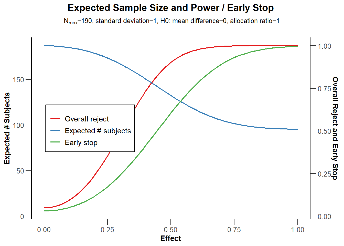
The following graph illustrates how the expected sample size changes with the true effect size in a design that includes stopping for both efficacy (early stop for large effects) and futility (early stop for null effects).

5. A Bayesian Decision-Theoretic Alternative

Your background includes Bayesian Decision Theory, which offers a more foundational approach to this problem. Instead of pre-specifying error rates, a Bayesian approach defines a utility function that explicitly models the trade-offs. For example, utility could be the number of true discoveries minus the cost of data collection. The optimal rule is then to stop when the expected utility of stopping exceeds the expected utility of continuing for one more batch of data.

While we will proceed with the more common frequentist alpha-spending framework for your pre-registration, it's valuable to recognize that this decision-theoretic perspective provides a powerful, first-principles justification for the logic of sequential analysis. The core idea is the same: making a principled, pre-specified decision based on the expected value of more information.

6. Defining the Stopping Rule for Your Experiment

Now, let's synthesize these concepts into a concrete stopping rule for your proposed N-of-1 crossover experiment. This is the kind of specific statement you will need for your pre-registration document.

For each experimental period (e.g., comparing "Nesting" vs. "Separate A"), you will collect daily satisfaction scores for, say, 12 weeks.

Proposed Stopping Rule:

Data collection within each 12-week experimental period will follow a group sequential design. We will perform two interim analyses at 4 weeks and 8 weeks, in addition to the final analysis at 12 weeks.

1. Spending Functions: We will use an O'Brien-Fleming-like alpha-spending function for efficacy and a Pocock-like beta-spending function for futility, with an overall two-sided $\alpha =0.05$ and $\beta =0.20$ (80% power).
2. Efficacy Boundary: At an interim analysis, if the p-value for the primary outcome (change in Triadic Satisfaction Index) is less than the pre-specified O'Brien-Fleming boundary for that look, the period will be terminated, and the intervention will be considered effective for that period.
3. Futility Boundary: If the p-value exceeds the pre-specified Pocock futility boundary (i.e., the data are highly consistent with the null hypothesis), the period will be terminated for futility.
4. Continuation: If the p-value falls between the efficacy and futility boundaries, data collection will continue to the next scheduled look.
5. Implementation: All boundaries will be calculated prior to the start of the experiment using the rpact package in R, and these exact p-value thresholds will be included in the pre-registration. The decision to perform an interim analysis is fixed by this schedule and is not contingent on the data observed.

This rule is robust because the stopping criteria are not based on an arbitrary p-value threshold but on pre-calculated boundaries that preserve the overall error rates of the study. The flexibility of rpact and alpha-spending functions also allows for adjustments if, for logistical reasons, a look is performed with a slightly different amount of data than planned.

Conclusion

In this lesson, we have constructed a framework for designing data collection stopping rules that are both efficient and statistically rigorous. By moving from ad-hoc optional stopping to principled sequential analysis, we can look at our data during an experiment without compromising the integrity of our final conclusions.

Key Takeaways:

• Optional Stopping vs. Sequential Analysis: Repeatedly checking data against a fixed alpha (e.g., 0.05) inflates the Type I error rate. Sequential analysis pre-specifies a limited number of "looks" and adjusts the significance thresholds to control the overall error rate.
• Alpha-Spending Functions: These are pre-specified strategies for distributing the total Type I error budget across interim analyses. O'Brien-Fleming is conservative early on, while Pocock gives a higher chance of stopping early.
• Stopping for Futility: In addition to stopping for efficacy (success), we can pre-specify rules to stop early if the data strongly suggest there is no meaningful effect, improving overall efficiency.
• Pre-registration is Crucial: The entire plan—the number of looks, the spending functions, and the precise boundaries—must be defined before the experiment begins and documented in a pre-registration.

You are now equipped to define a critical component of your experimental protocol. In our next and final lesson for this module, we will bring everything together—the analysis plan, the handling of multiple comparisons, the HARKing prevention strategy, and these stopping rules—to draft the complete pre-registration document for your proposed triadic experiment.