Interventional Distributions in Triadic Systems with Interference

Introduction

In our last lesson, we adapted the backdoor criterion to handle causal interference, enabling us to identify valid adjustment sets in system-level DAGs. This was a crucial step, but the backdoor criterion is only one tool in our arsenal. It works when we can observe and condition on a set of variables that blocks all non-causal paths, but what happens when a key confounder is unmeasurable?

This lesson introduces a more powerful and complete framework for causal identification: Judea Pearl's do-calculus. We will move beyond simple adjustment and learn a set of formal rules that allow us to determine if a causal effect can be estimated from data, even in complex scenarios where the backdoor criterion fails. Our primary goal is to understand how to derive the interventional distribution, $P (Y ∣ do (T))$ , which represents the distribution of an outcome $Y$ had we forced the treatment $T$ to take a specific value. For your study, this is the formal expression for questions like, "What would the pivot's satisfaction be if we assigned the triad to a specific living arrangement?"

1. The Interventional Distribution: Seeing vs. Doing

Before diving into the rules, it's essential to solidify the distinction between an observational conditional distribution, $P (Y ∣ T)$ , and an interventional distribution, $P (Y ∣ do (T))$ . Your statistics background makes you an expert in conditional probability, which describes beliefs updated by observation. Causal inference, however, is about the consequences of action.

$P (Recovery ∣ Treatment A)$ asks: "Among the patients who we observe taking Treatment A, what is the probability of recovery?" This is susceptible to confounding; for example, doctors might give Treatment A to sicker patients.
$P (Recovery ∣ do (Treatment A))$ asks: "If we forced every patient to take Treatment A, what would the probability of recovery be?" This represents a physical intervention on the system.

The following video lecture provides an excellent conceptual foundation for this distinction and introduces the formal language of Structural Causal Models (SCMs) that underpins it.

Lectures on Causality: Jonas Peters, Part 1

This excerpt from a lecture by Jonas Peters at the Broad Institute clearly explains the difference between observation and intervention and how SCMs model this difference.

Please watch the following segments: Prediction vs. Causality (this part): Focus on the gene expression example, which perfectly illustrates why observing a gene's activity is different from actively deleting it. Modeling Interventions (this segment): This is the crucial part. Pay close attention to how an intervention is mathematically modeled by replacing a structural equation in an SCM. This is the mechanism that generates the interventional distribution. The Do-Notation (this final part): This section formally introduces Pearl's do notation and emphasizes again why P(Y|\text{do}(X)) is not the same as P(Y|X).

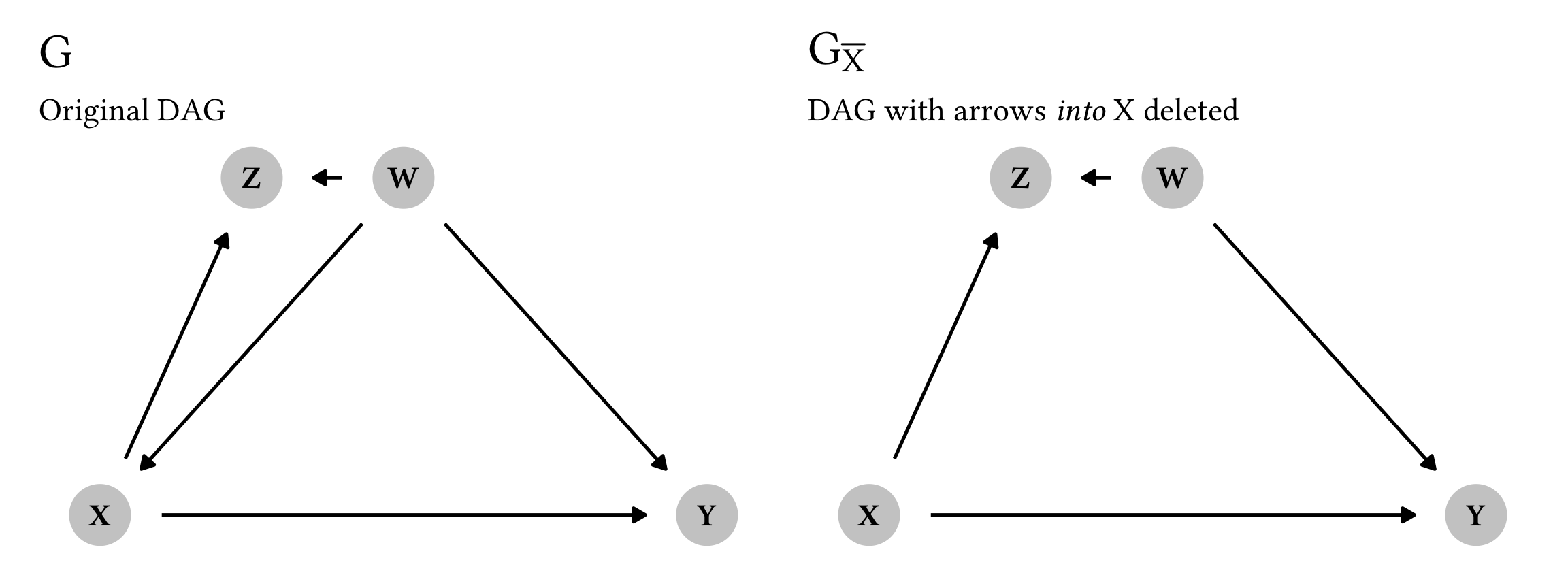
The key insight is that an intervention, represented by the do-operator, changes the data-generating process itself. Graphically, applying do(T=t) corresponds to "mutilating" the causal graph by deleting all incoming arrows to the treatment node $T$ and fixing its value to $t$ . The interventional distribution is simply the probability distribution that exists in this modified graph.

This diagram illustrates the goal of do-calculus. We start with a causal model and its implied observational distribution. An intervention creates a 'mutilated' model with a corresponding interventional distribution. Do-calculus provides the rules to find an 'estimable formula'—an expression using only observational probabilities—that is equivalent to the interventional distribution we want to find.

2. The Three Rules of Do-Calculus

Do-calculus consists of three rules for manipulating do-expressions. These rules are provably complete, meaning if a causal quantity is identifiable from the graph structure, it can be derived using these rules. They allow us to transform expressions containing do into expressions involving only standard conditional probabilities that can be estimated from data.

The video below provides a concise and clear walkthrough of each rule. The notation $G_{X ˉ}$ refers to the graph where arrows into X are removed, while $G_{X}$ refers to the graph where arrows out of X are removed.

5.4 - Pearl’s do-calculus

This video from Brady Neal's "Causal Inference" course is a standard reference for learning do-calculus. It breaks down each rule with clear examples.

Please watch from the beginning to the end. The video covers: The graph notation used (here). Rule 1: Insertion/deletion of observation (here). Rule 2: Action/observation exchange (here). Rule 3: Insertion/deletion of action (here). The completeness of the rules (here).

Let's summarize the rules in the context of our variables $T$ (treatment), $Y$ (outcome), $Z$ (another variable), and $W$ (a set of covariates).

Rule 1: Ignoring Irrelevant Observations

Formula: $P (Y ∣ do (T), Z, W) = P (Y ∣ do (T), W)$ if $(Y ⊥ Z ∣ T, W)_{G_{T ˉ}}$
Intuition: If observing $Z$ provides no additional information about $Y$ in a world where we've already fixed $T$ (and are observing $W$ ), then we can ignore $Z$ . This rule helps simplify expressions.

Rule 2: The Backdoor Criterion Generalized

Formula: $P (Y ∣ do (T), W) = P (Y ∣ T, W)$ if $(Y ⊥ T ∣ W)_{G_{T}}$
Intuition: This is the backdoor rule. If $W$ blocks all backdoor paths from $T$ to $Y$ , then intervening on $T$ is the same as conditioning on $T$ . The notation $G_{T}$ (graph with outgoing arrows from T removed) is a graphical way to check the backdoor criterion: if $Y$ and $T$ are d-separated by $W$ in this modified graph, the rule applies.

An example of graph mutilation for Rule 2. To check if we can swap `do(X)` with `X`, we assess d-separation in the graph G with outgoing arrows from X deleted. This is equivalent to checking the backdoor criterion in the original graph G.

Rule 3: Removing an Intervention

Formula: $P (Y ∣ do (T), W) = P (Y ∣ W)$ if $(Y ⊥ T ∣ W)_{G_{T ˉ, Z ˉ}}$ where $Z$ are non-ancestors of $Y$ in $G_{T ˉ}$ .
Intuition: This is the most powerful rule, often used when unobserved confounding is present. If there are no causal paths from $T$ to $Y$ in the manipulated graph, we can remove the intervention do(T) altogether. This rule is the key to solving problems like the front-door adjustment.

3. Applying Do-Calculus to Systems with Interference

The rules of do-calculus are universal. They don't change in the presence of interference. What does change is the graph we apply them to. As established in the previous lesson, we must use a system-level DAG that explicitly models the interference pathways. The "treatment" becomes the vector of treatments for the whole group, $T$ , and the rules are applied to identify effects like $P (Y_{A} ∣ do (T))$ .

Formal research in network causal inference provides the theoretical grounding for this approach. While highly technical, the following paper confirms that do-calculus is the correct tool for identification in these complex relational models.

[PDF] Inferring individual direct causal effects under heterogeneous peer ...

This paper develops a framework called the Network Structural Causal Model (NSCM) to handle interference. We won't delve into the full details, but its conclusion on identification is directly relevant.

First, quickly skim section 4. Network structural causal model (NSCM) to see how the authors extend SCMs to network settings, creating a "Network Abstract Ground Graph" (NAGG) to reason about dependencies. Then, carefully read the short subsection on identification. The key result is Corollary 4, which states that the counterfactual term (equivalent to our interventional distribution) can be identified from data if certain conditions hold. The final sentence of the proof's summary is what matters for us: it "follows from do-calculus applied to NAGG." This confirms that the rules you just learned are precisely the engine for identification in your triadic system.

A Concrete Example: Front-Door Adjustment with Interference

Let's illustrate this with a practical scenario that extends beyond last lesson's backdoor adjustment. Imagine in your vee-triad study, there's an unobserved shared confounder, Household_Tension ( $U$ ), which affects both the chosen living arrangement ( $T_{A}$ ) and the pivot's satisfaction ( $Y_{A}$ ).

DAG: $T_{A} \leftarrow U \to Y_{A}$ .
Problem: Because $U$ is unobserved, we cannot use the backdoor criterion (Rule 2) to identify $P (Y_{A} ∣ do (T_{A}))$ , as we can't condition on $U$ .

However, suppose the effect of the living arrangement on satisfaction is fully mediated through an observed variable, such as the pivot's Sense_of_Autonomy ( $M$ ).

Full path: $T_{A} \to M \to Y_{A}$ .
Assumptions for front-door:
1. $M$ intercepts all directed paths from $T_{A}$ to $Y_{A}$ .
2. There is no unblocked backdoor path from $T_{A}$ to $M$ .
3. All backdoor paths from $M$ to $Y_{A}$ are blocked by $T_{A}$ .

Our goal is to find an estimable expression for $P (Y_{A} ∣ do (T_{A}))$ . Here is a sketch of the derivation using do-calculus:

Start with the target: $P (Y_{A} ∣ do (T_{A}))$
Introduce the mediator $M$ : We can sum over $M$ .
$P (Y_{A} ∣ do (T_{A})) = \sum_{m} P (Y_{A} ∣ m, do (T_{A})) P (m ∣ do (T_{A}))$
Analyze the first term, $P (Y_{A} ∣ m, do (T_{A}))$ : The backdoor path from $M$ to $Y_{A}$ is $M \leftarrow T_{A} \leftarrow U \to Y_{A}$ . This path is blocked by conditioning on $T_{A}$ . So, we can apply Rule 2 to swap do(T_A) for conditioning on T_A.
$P (Y_{A} ∣ m, do (T_{A})) = P (Y_{A} ∣ m, T_{A})$
Analyze the second term, $P (m ∣ do (T_{A}))$ : By assumption, there is no backdoor path from $T_{A}$ to $M$ . So we can apply Rule 2 again.
$P (m ∣ do (T_{A})) = P (m ∣ T_{A})$
Substitute back:
$P (Y_{A} ∣ do (T_{A})) = \sum_{m} P (Y_{A} ∣ m, T_{A}) P (m ∣ do (T_{A}))$
This gives the first part of the front-door formula. To get the final form, we must express $P (m ∣ do (T_{A}))$ using $P (T_{A})$ . A few more steps involving Rule 3 would lead to the full front-door formula:
$P (Y_{A} ∣ do (T_{A})) = \sum_{m} P (m ∣ T_{A}) \sum_{t_{A}^{'}} P (Y_{A} ∣ m, T_{A} = t_{A}^{'}) P (T_{A} = t_{A}^{'})$
This final expression contains no do-operators. Every term is an observational probability you can estimate from your data. This demonstrates how do-calculus allows us to identify a causal effect even when a crucial confounder is unobserved.

Conclusion

Today we have moved from the specific case of the backdoor criterion to the general and complete system of do-calculus. This provides you with the formal machinery to assess causal identifiability in any causal graph, no matter how complex.

Key Takeaways:

The interventional distribution $P (Y ∣ do (T))$ describes the outcome distribution after a physical intervention, which is modeled by mutilating the causal graph.
Do-calculus provides three formal rules to manipulate do-expressions and, if the effect is identifiable, convert them into estimable expressions of observational data.
These rules apply directly to complex systems with interference; the logic is the same, but the graph it operates on must represent the entire interacting system.
We can use do-calculus to derive identification strategies like the front-door adjustment, which work even when unobserved confounders prevent the use of the simple backdoor criterion.

In our next lesson, we will apply these powerful identification tools to our primary research questions. We will use the principles of the backdoor criterion and do-calculus to formally determine whether we can separately identify the direct effect of a treatment on an individual and the indirect spillover effects from their partners' treatments.