Introduction
In our previous lesson, we developed a powerful tool, the E-value, to assess how robust our causal estimates are to potential unmeasured confounding. This allowed us to quantify the strength of a hypothetical unmeasured variable that would be needed to nullify our findings. However, that analysis was performed under the assumption that our chosen causal model—the DAG and its corresponding regression equation—was correctly specified.
Today, we take a step back to challenge an even more fundamental assumption: the model structure itself. In any complex analysis, researchers face a "garden of forking paths," a series of decisions about which variables to include, how to measure them, and what functional forms to assume. Each set of choices represents a different, often equally plausible, structural model. This lesson addresses the critical learning outcome: to evaluate the robustness of causal conclusions to alternative structural model specifications. We will move beyond sensitivity to a single parameter and explore how to systematically assess whether our conclusions hold across a "multiverse" of reasonable analyses.
The Problem of Model Specification
A Structural Causal Model (SCM) is a formal representation of our assumptions about how the world works. As you know from your background in causal analysis, the identification of a causal effect via methods like the backdoor adjustment is entirely dependent on the assumed causal graph. An incorrect graph can lead to profoundly incorrect conclusions.
For instance, including a collider in an adjustment set, a common specification error, can induce spurious associations and bias your estimate. The choice of which covariates to include is not merely a statistical decision but a causal one, predicated on the assumed structure of the DAG.
To see a concrete example of this, let's revisit a segment from Brady Neal's course on causal models.
Watch the clip from this example on the effect of sodium on blood pressure. Notice how three different adjustment sets—which correspond to three different underlying model specifications—produce errors ranging from 407% to 19% to just 0.02%. This clearly illustrates that the choice of specification is not a minor detail; it is fundamental to the validity of the causal estimate.
In our vee-triad experiment, we face dozens of such choices:
- Which potential confounders (e.g., financial stress, work schedules, shared hobbies) should be in our final model?
- How should we operationalize our outcome? Should we use the composite triadic satisfaction index, the pivot's satisfaction, or an average of all members?
- Should we assume a linear relationship between the living arrangement and satisfaction, or test for non-linearities?
- Should we exclude experimental periods where a major external event occurred?
Selectively reporting the results from the one combination of choices that yields a favorable outcome is a major threat to scientific credibility. The solution is not to pretend these choices don't exist, but to confront them transparently.
A Systematic Solution: Specification Curve Analysis
Specification Curve Analysis (SCA) offers a systematic and transparent method for dealing with the multiplicity of analytical choices. Instead of presenting a single "preferred" model, SCA involves estimating the effect of interest across a large set of defensible specifications and visualizing the results.
The foundational paper by Simonsohn, Simmons, and Nelson provides the conceptual framework for this powerful technique. Given your statistical background, you will appreciate its formal treatment of the problem.
[PDF] Specification curve analysis - Wharton Faculty Platform
Let's begin with the paper that formalized this approach to understand the 'why' before we get to the 'how'.
First, read the introduction to grasp the core problem of arbitrary and motivated analytical decisions. Then, focus on the section "A formal presentation of the problem". This frames the issue in precise statistical terms, characterizing the handful of specifications reported in a paper (π) as a small, curated, and non-independent sample of the entire universe of reasonable specifications (Π).
Implementing and Visualizing the "Multiverse"
The output of an SCA is a two-part plot. The top panel shows the distribution of the coefficient estimate across all specifications, while the bottom panel is a dashboard indicating which modeling choices correspond to each estimate. This allows us to instantly see how sensitive our results are to particular choices.
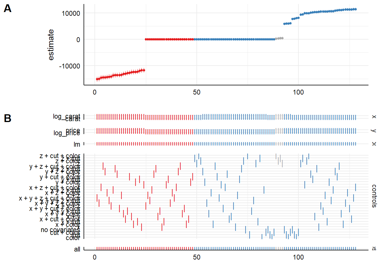
To implement this, we can use tools like the starbility package in R, which is designed to construct these analyses systematically. The "researcher degrees of freedom" we identified in our pre-registration module become the inputs that define our specification multiverse.
42 Sensitivity Analysis and Robustness Checks - Bookdown
Now let's turn to a practical guide for implementation. This chapter from "A Guide on Data Analysis" provides excellent R code examples using the starbility package.
Begin by reading "The Philosophy of Robustness" to solidify the concept. Then, dive into the main section on "Specification Curve Analysis," which introduces the two-panel visualization. Finally, carefully study the subsection "Basic Specification Curve with Multiple Controls." Don't worry about running the code right now; instead, focus on understanding how the base_controls, perm_controls, and perm_fe_controls are defined to build the "multiverse" of models. This is precisely the logic you would use to map your analytical choices from our triad experiment into a systematic analysis.
When interpreting the resulting curve for our triad experiment, we would ask:
- Does the estimated effect of our "living together" intervention remain consistently positive across most specifications?
- Do the confidence intervals for most specifications exclude zero?
- Are the significant, large effects driven by one or two specific modeling choices (e.g., only when we exclude financial stress as a control), or are they broadly distributed?
Inferential Specification Curve Analysis
SCA is more than just a descriptive visualization; it provides a framework for joint hypothesis testing. Since the different specifications are not statistically independent, we cannot simply count the number of significant results. The correct approach, as you might anticipate from your background in computational statistics, involves resampling.
[PDF] Specification curve analysis - Wharton Faculty Platform
Let's return to the Simonsohn et al. paper to see how the formal inferential component of SCA works.
Quickly review Step 2 in the paper to see the descriptive curve for the famous hurricane names study (Step 2). Then, read Step 3, "Inference with specification curve analysis," with care. Focus on the three proposed test statistics (median effect, share of significant results, aggregated Z-score) and the logic of using resampling (shuffling the treatment variable in an experimental context) to generate the distribution of these statistics under the null hypothesis of no effect.
By comparing the curve from our actual data to the distribution of curves generated from hundreds of resampled datasets where the null is true by construction, we can calculate a single, valid p-value for the joint evidence across all specifications. This transforms a sea of potentially cherry-picked results into a single, robust statistical test.
Other Robustness and Refutation Checks
SCA is a cornerstone of model robustness, but it's part of a broader family of "refutation" tests designed to probe a model for weaknesses. In the absence of a ground-truth test set for a causal question, these checks are our primary defense against invalid conclusions.
Other common refutation methods include:
- Placebo Treatment: Replace the actual treatment variable with a random variable that should have no effect (e.g., a randomly generated number). If your full analytical pipeline still produces a "significant" effect, it indicates a flaw in the model or estimation procedure.
- Adding a Simulated Confounder: This method provides a nice bridge from our previous lesson on E-values. You can explicitly add a new, simulated confounder node to your DAG with varying degrees of association with the treatment and outcome. You then re-run the analysis to see how strong this simulated confounder must be to alter your conclusion. This is a direct test of robustness to a specific kind of misspecification—a missing variable.
Foundations of causal inference and its impacts on machine learning webinar
This validation step is a core part of any rigorous causal analysis. This clip from a Microsoft Research talk on their DoWhy library provides a great summary of different refutation methods.
Please watch the segment from this point. Pay attention to the distinction between "unit tests" and "integration tests," and focus on the intuition behind the placebo treatment refuter and the sensitivity analysis for unobserved confounding. These methods provide a way to actively audit your model's credibility.
Conclusion
Today we have expanded our toolkit for assessing the credibility of our causal claims. While the previous lesson focused on the threat of unmeasured variables within a given model, this lesson tackled the threat of the model specification itself.
Key Takeaways:
- A causal conclusion is always conditional on the assumed Structural Causal Model (SCM). Different plausible modeling choices lead to a "multiverse" of potential results.
- Specification Curve Analysis (SCA) provides a systematic and transparent method to estimate an effect across many defensible model specifications, protecting against selective reporting.
- SCA is both a descriptive tool for visualizing the stability of an effect and an inferential tool that allows for joint hypothesis testing via resampling methods.
- Broader refutation checks, such as placebo tests and adding simulated confounders, are essential for building confidence in a causal claim by actively trying to prove it wrong.
In our final lesson, we will perform the ultimate step of our project: synthesis. We will bring together the results from our experimental design, our primary regression model, the E-value sensitivity analysis, and the specification curve analysis. Our goal will be to construct a single, coherent causal narrative that determines the optimal living arrangement for the triad and, crucially, articulates the evidence-backed causal mechanisms responsible for its effectiveness.