Yang-Mills Theory: Field Strength Tensor and Lagrangian

Welcome back to our exploration of gauge theories. In the previous lesson, we embarked on a significant generalization, moving from the abelian U(1) symmetry of QED to non-abelian SU(N) symmetries. By enforcing the principle of local gauge invariance, we were compelled to introduce a set of matrix-valued gauge potentials, $A_{μ} = A_{μ}^{a} T^{a}$ , and to replace the ordinary derivative with a covariant derivative, $D_{μ} = \partial_{μ} - i g A_{μ}$ . This process not only restored the symmetry of our matter Lagrangian but also naturally introduced an interaction term, $g ψ ˉ γ^{μ} A_{μ} ψ$ , describing how matter couples to the gauge fields.

However, our work is incomplete. The gauge fields we introduced are currently just background fields without any dynamics of their own. They have no kinetic term in the Lagrangian that would describe their propagation and evolution. Our goal in this lesson is to rectify this by constructing a fully gauge-invariant kinetic term for the $A_{μ}$ fields. This will lead us directly to the celebrated Yang-Mills Lagrangian, the foundation of the modern description of the fundamental forces. In doing so, we will uncover a profound new feature: the self-interaction of gauge bosons.

The Quest for a Gauge-Invariant Kinetic Term

In electromagnetism, the kinetic term for the photon field $A_{μ}$ is built from the field strength tensor, $F_{μν} = \partial_{μ} A_{ν} - \partial_{ν} A_{μ}$ . The Maxwell Lagrangian, $L = - \frac{1}{4} F_{μν} F^{μν}$ , is both a Lorentz scalar and gauge invariant. Can we do something similar for the non-abelian case?

We cannot simply use $\partial_{μ} A_{ν}^{a} - \partial_{ν} A_{μ}^{a}$ . A quick check shows that this expression does not transform covariantly under the non-abelian gauge transformation we derived. We need a more sophisticated object that properly respects the SU(N) symmetry at every point.

The key insight comes from the very tool we invented to handle the local symmetry: the covariant derivative. In differential geometry, the commutator of covariant derivatives measures the curvature of the space. In our context, it will measure the "field strength" of our gauge connection. Let's compute the commutator $[D_{μ}, D_{ν}]$ acting on a matter field $ψ$ .

[D_{μ}, D_{ν}] ψ = (D_{μ} D_{ν} - D_{ν} D_{μ}) ψ

Let's expand the first term:

D_{μ} D_{ν} ψ = (\partial_{μ} - i g A_{μ}) (\partial_{ν} - i g A_{ν}) ψ = \partial_{μ} \partial_{ν} ψ - i g (\partial_{μ} A_{ν}) ψ - i g A_{ν} (\partial_{μ} ψ) - i g A_{μ} (\partial_{ν} ψ) + (i g)^{2} A_{μ} A_{ν} ψ

Now we write out the second term, $D_{ν} D_{μ} ψ$ , by simply swapping the indices $μ \leftrightarrow ν$ . When we subtract the two, the symmetric term $\partial_{μ} \partial_{ν} ψ$ cancels, as do the terms involving derivatives of $ψ$ . We are left with:

[D_{μ}, D_{ν}] ψ = - i g (\partial_{μ} A_{ν} - \partial_{ν} A_{μ}) ψ - g^{2} (A_{μ} A_{ν} - A_{ν} A_{μ}) ψ = - i g (\partial_{μ} A_{ν} - \partial_{ν} A_{μ} - i g [A_{μ}, A_{ν}]) ψ

This calculation reveals that the commutator of covariant derivatives is not zero. Instead, it is equivalent to multiplication by a new matrix-valued object. We define this object as the non-abelian field strength tensor, $F_{μν}$ :

F_{μν} = \partial_{μ} A_{ν} - \partial_{ν} A_{μ} - i g [A_{μ}, A_{ν}]

With this definition, we can write the commutator relation compactly:

[D_{μ}, D_{ν}] = - i g F_{μν}

Notice the crucial new piece: the commutator $- i g [A_{μ}, A_{ν}]$ . This term is a direct consequence of the non-abelian nature of the group (i.e., the fact that the generators $T^{a}$ do not commute). If the group were abelian like U(1), this term would vanish, and we would recover the familiar electromagnetic field strength tensor. This non-linear term is the source of the rich physics of Yang-Mills theory.

The video below provides a very clear derivation of this result and explains its significance.

The Transformation Property of $F_{μν}$

Now that we have our candidate for the field strength, we must determine how it transforms under a gauge transformation $ψ \to U (x) ψ$ . We could substitute the transformation rule for $A_{μ}$ into the definition of $F_{μν}$ and compute directly, but this is algebraically intensive. A far more elegant path is to use the commutator definition.

We know that the covariant derivative is designed to transform "homogeneously": $(D_{μ} ψ)^{'} = U (D_{μ} ψ)$ . Applying this twice, we find how the commutator transforms:

([D_{μ}, D_{ν}] ψ)^{'} = U ([D_{μ}, D_{ν}] ψ)

Now, let's substitute our definitions $[D_{μ}, D_{ν}] = - i g F_{μν}$ and $([D_{μ}, D_{ν}] ψ)^{'} = (- i g F_{μν}^{'}) ψ^{'} = (- i g F_{μν}^{'}) U ψ$ :

(- i g F_{μν}^{'}) U ψ = U (- i g F_{μν}) ψ

Canceling $- i g$ and $ψ$ and multiplying by $U^{- 1} = U^{†}$ from the right, we arrive at the transformation law for the field strength tensor:

F_{μν}^{'} (x) = U (x) F_{μν} (x) U^{†} (x)

This is a remarkable result. Unlike the gauge potential $A_{μ}$ , which transforms inhomogeneously, the field strength $F_{μν}$ transforms in a simple, homogeneous way. This type of transformation, where an object is conjugated by the group element, is known as transforming in the adjoint representation of the gauge group.

This simple transformation property is exactly what we need to construct an invariant quantity.

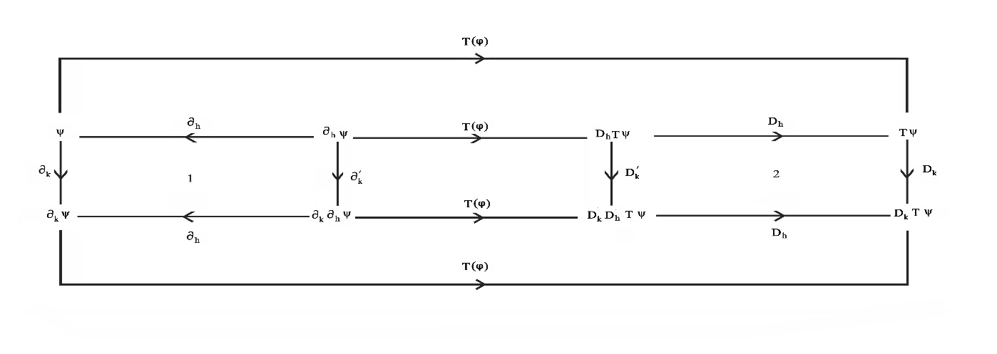
The following diagram offers a more abstract, geometric perspective on the origin of the field strength (or curvature). It illustrates that while partial derivatives commute (path '1'), covariant derivatives do not (path '2'). The "failure" of the diagram to close for covariant derivatives is precisely measured by the curvature, $F_{μν}$ .

This commutative diagram illustrates the concept of curvature. The inner square (1) shows that for ordinary partial derivatives, the order of application does not matter: $\partial_k \partial_h \psi = \partial_h \partial_k \psi$. The outer square (2) involves covariant derivatives $D_k$ and $D_h$. The fact that $D_k D_h T\psi \neq D_h D_k T\psi$ indicates that the 'space' has curvature. This curvature is the field strength, arising from the non-commutativity of the covariant derivatives.

The Yang-Mills Lagrangian

We are now ready to build our Lagrangian. We need a Lorentz-scalar, gauge-invariant kinetic term from $F_{μν}$ . Since $F_{μν}$ is a matrix, we cannot simply square it. However, we can construct a scalar using the trace. Consider the quantity $Tr (F_{μν} F^{μν})$ . Let's see how it behaves under a gauge transformation:

Tr (F_{μν}^{'} F^{' μν}) = Tr ((U F_{μν} U^{†}) (U F^{μν} U^{†}))

Using the cyclic property of the trace, $Tr (A B C) = Tr (C A B)$ , we can move the final $U^{†}$ to the front:

Tr (F_{μν}^{'} F^{' μν}) = Tr (U^{†} U F_{μν} U^{†} U F^{μν}) = Tr (F_{μν} F^{μν})

The quantity is invariant! We have found our kinetic term. The standard convention for the Yang-Mills Lagrangian is:

L_{YM} = - \frac{1}{2} Tr (F_{μν} F^{μν})

The normalization factor can vary between texts. If we expand this using $A_{μ} = A_{μ}^{a} T^{a}$ and use the standard normalization for the generators $Tr (T^{a} T^{b}) = \frac{1}{2} δ^{ab}$ , we get the form more commonly seen in component notation:

L_{YM} = - \frac{1}{4} F_{μν}^{a} F_{a}^{μν}

where $F_{μν}^{a}$ are the components of the field strength tensor in the Lie algebra basis:

F_{μν}^{a} = \partial_{μ} A_{ν}^{a} - \partial_{ν} A_{μ}^{a} + g f^{ab c} A_{μ}^{b} A_{ν}^{c}

Here, $f^{ab c}$ are the structure constants of the Lie algebra, defined by $[T^{b}, T^{c}] = i f^{ab c} T^{a}$ .

For a detailed walkthrough of these final steps, the following resources are excellent. The text from David Tong's lecture notes provides a very compact and clear summary, while the videos offer a more narrative explanation.

Advanced quantum field theory, Lecture 11

This is a more advanced lecture from Tobias Osborne that goes into great detail on the construction of the theory. Given your background, you may find the depth here rewarding.

Watch the following two segments: The Field Strength from Commutators: Here, the lecturer derives the field strength (which he calls curvature) from the commutator of covariant derivatives, explicitly writing out the component form and highlighting the new quadratic term in the gauge field. Building the Lagrangian: This part shows how to construct the invariant Lagrangian using the trace and discusses the crucial physical consequence: the appearance of cubic and quartic self-interaction terms for the gauge bosons.

The Physics of Self-Interaction

Let's examine the physical implication of our final Lagrangian. When we substitute the definition of $F_{μν}^{a}$ into $L_{YM} = - \frac{1}{4} F_{μν}^{a} F_{a}^{μν}$ , the term $g f^{ab c} A_{μ}^{b} A_{ν}^{c}$ leads to profound consequences.

L_{YM} = - \frac{1}{4} (\partial_{μ} A_{ν}^{a} - \partial_{ν} A_{μ}^{a}) (\partial^{μ} A^{ν a} - \partial^{ν} A^{μ a}) - \frac{g}{2} f^{ab c} (\partial_{μ} A_{ν}^{a} - \partial_{ν} A_{μ}^{a}) A^{μ b} A^{ν c} - \frac{g ^{2}}{4} f^{ab c} f^{a d e} A_{μ}^{b} A_{ν}^{c} A^{μ d} A^{ν e}

The first term is the standard kinetic term, just like in QED. But the second and third terms are new:

A cubic interaction term, proportional to $g$ , describing three gauge bosons interacting at a vertex.
A quartic interaction term, proportional to $g^{2}$ , describing four gauge bosons interacting at a vertex.

This is the central physical difference between abelian and non-abelian gauge theories. In QED, photons do not carry charge, so they do not interact with each other directly (Maxwell's equations are linear). In contrast, the gauge bosons of a non-abelian theory, like the gluons of QCD, do carry the "charge" of the interaction they mediate (color charge). Therefore, they interact with themselves. This self-interaction is responsible for many of the unique phenomena in the theory of the strong force, such as asymptotic freedom and color confinement.

Conclusion

In this lesson, we have completed the construction of the classical Yang-Mills theory. By seeking a dynamic term for the gauge fields, we were led to the non-abelian field strength tensor and, ultimately, to a unique, gauge-invariant Lagrangian.

Key Takeaways:

The non-abelian field strength tensor $F_{μν}$ is defined via the commutator of covariant derivatives: $[D_{μ}, D_{ν}] = - i g F_{μν}$ .
Its explicit form, $F_{μν} = \partial_{μ} A_{ν} - \partial_{ν} A_{μ} - i g [A_{μ}, A_{ν}]$ , contains a non-linear term that is the hallmark of non-abelian theories.
$F_{μν}$ transforms homogeneously under gauge transformations ( $F_{μν}^{'} = U F_{μν} U^{†}$ ), allowing for the construction of an invariant kinetic term.
The Yang-Mills Lagrangian, $L_{YM} = - \frac{1}{2} Tr (F_{μν} F^{μν})$ , is the unique, Lorentz-invariant, and gauge-invariant Lagrangian describing the dynamics of the gauge fields.
A direct consequence of the non-linear term in $F_{μν}$ is that non-abelian gauge bosons self-interact, leading to cubic and quartic interaction vertices in the theory.

We now have a complete classical field theory for both matter and gauge fields, fully respecting local non-abelian gauge invariance. The total Lagrangian is $L = ψ ˉ (i γ^{μ} D_{μ} - m) ψ + L_{YM}$ .

Preview of the Next Lesson:

Having established the classical theory, our next challenge is to quantize it. As you know from QED, quantization of gauge theories is subtle due to the redundancy of the description (gauge freedom). In the non-abelian case, this subtlety becomes a major technical hurdle. The self-interaction of the gauge fields complicates the standard procedures. In our next lesson, we will discuss the necessity of gauge fixing and introduce the Faddeev-Popov ghost fields, which are an essential mathematical tool for correctly quantizing Yang-Mills theories using the path integral formalism.

Recommended resources

The Quest for a Gauge-Invariant Kinetic Term

The Transformation Property of Fμν​

The Yang-Mills Lagrangian

The Physics of Self-Interaction

Conclusion

The Transformation Property of $F_{μν}$