Shortest Paths in Weighted DAGs: DP on Topological Order

1. Shortest Paths as a Dynamic Programming Problem

Just like counting paths, the problem of finding the shortest path in a DAG has the two key properties that make it suitable for dynamic programming:

• Optimal Substructure: The shortest path from a source s to a vertex v must pass through one of v's immediate predecessors. The subpath to that predecessor must itself be a shortest path.
• Overlapping Subproblems: The shortest path to a vertex u might be needed to compute the shortest paths for several other vertices that u points to.

Let's formalize this. We can define our DP state as:
dist[v] = The length of the shortest path from the source vertex s to vertex v.

Our goal is to compute dist[v] for all v in the graph. The recurrence relation arises from the optimal substructure property. To get to v, we must have arrived from some predecessor u via the edge (u, v). The total path length would be dist[u] + weight(u, v). Since we want the shortest path, we must choose the predecessor u that minimizes this value.

This gives us the following recurrence relation:

The base case is for the source vertex s, where the distance to itself is 0: dist[s] = 0. For all other vertices v, we initialize their distances to infinity (dist[v] = ∞) to signify they are not yet reached.

Notice the striking similarity to the path-counting recurrence from the last lesson, dp[v] = Σ dp[u]. We've simply replaced summation with the min operation and incorporated the edge weights.

The following resources provide a more formal perspective on this DP formulation. The MIT video, in particular, frames this problem beautifully within a general DP framework.

2. The Algorithm: Relaxation via Topological Sort

Having established the DP recurrence, the question remains: in what order should we compute the dist values? As you've probably guessed, a topological sort is the answer. By processing vertices in topological order, we ensure that by the time we need to calculate dist[v], we have already finalized the shortest path distances for all of its predecessors.

This allows for a simple, iterative algorithm:

1. Initialize: Create a dist array of size V. Set dist[source] = 0 and all other entries to INF.
2. Topological Sort: Find a topological ordering of the graph's vertices. You can use either Kahn's algorithm or a DFS-based approach.
3. Iterate and Relax: Go through each vertex u in the computed topological order. For each outgoing edge (u, v) with weight w:
   • Check if we've found a shorter path to v by going through u.
   • This update step is called relaxation: if (dist[u] + w < dist[v]), then update dist[v] = dist[u] + w.

The term "relaxation" comes from the idea that we are gradually "relaxing" the distance estimates from their initial infinite values down to their true shortest path lengths.

The following resource from GeeksforGeeks outlines this process clearly.

3. A Visual Walkthrough

Let's trace the algorithm on an example. The image below shows a weighted DAG. The vertices are labeled r, s, t, x, y, z. Let's find the shortest paths from source s.

A valid topological sort of this graph is r, s, t, x, y, z. (Note: r comes before s because it's processed first in the traversal, but s has no incoming edges in this subgraph, so it could also come first). Let's assume our topological sort is s, t, x, y, z (ignoring r as it's unreachable from s).

1. Initialization: dist array = [∞, 0, ∞, ∞, ∞, ∞] for (r, s, t, x, y, z).

2. Topological Iteration:

   • Process s: dist[s] is 0.
     • Relax edge (s, t): dist[t] = min(∞, dist[s] + 2) = 2.
     • Relax edge (s, x): dist[x] = min(∞, dist[s] + 6) = 6.
     • dist is now [∞, 0, 2, 6, ∞, ∞]. (See image (d))
   • Process t: dist[t] is 2.
     • Relax edge (t, x): dist[x] = min(6, dist[t] + 7) = min(6, 2+7) = 6. No change.
     • Relax edge (t, y): dist[y] = min(∞, dist[t] + 4) = 6.
     • Relax edge (t, z): dist[z] = min(∞, dist[t] + 2) = 4.
     • dist is now [∞, 0, 2, 6, 6, 4]. (See image (e))
   • Process x: dist[x] is 6.
     • Relax edge (x, y): dist[y] = min(6, dist[x] - 1) = min(6, 6-1) = 5. Note the negative weight!
     • dist is now [∞, 0, 2, 6, 5, 4]. (See image (f))
   • Process y: dist[y] is 5.
     • Relax edge (y, z): dist[z] = min(4, dist[y] - 2) = min(4, 5-2) = 3. Again, a negative weight.
     • dist is now [∞, 0, 2, 6, 5, 3]. (See image (g))
   • Process z: No outgoing edges. (Image (h) shows the final state)

Final dist array from source s: s=0, t=2, x=6, y=5, z=3. Unreachable nodes like r remain ∞.

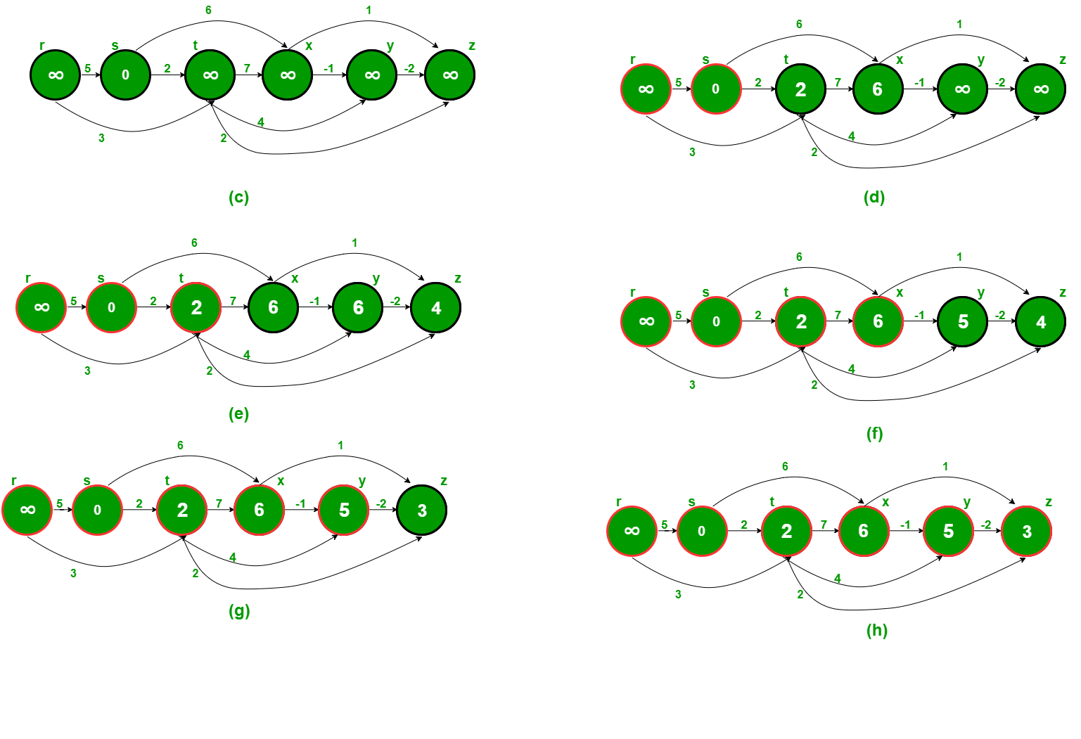
To see this process in action with a more detailed commentary, the following video provides an excellent dry run.

4. Implementation and Complexity

The C++ implementation is a direct translation of the algorithm. It involves a graph representation that supports weights (e.g., vector<pair<int, int>>), a function for topological sort, and the main loop that iterates and relaxes edges.

Complexity Analysis

• Time Complexity: The topological sort takes $O(V+E)$ time. The main loop iterates through each of the $V$ vertices once. The inner loop relaxes the outgoing edges of each vertex. Over the course of the entire algorithm, each edge is relaxed exactly once. Therefore, the relaxation phase also takes $O(V+E)$ time. The total time complexity is $O(V+E)$.
• Space Complexity: Storing the graph requires $O(V+E)$ space. The dist array, visited array, and the stack for topological sort require an additional $O(V)$ space. The total space complexity is $O(V+E)$.

This linear time complexity makes this algorithm exceptionally fast, outperforming general-purpose algorithms like Dijkstra's ($O(E\log V)$) or Bellman-Ford ($O(VE)$) on the specific case of DAGs.

Conclusion

You have now mastered a fundamental and highly efficient pattern: applying dynamic programming on a topologically sorted DAG. You've seen it work for both counting paths and, now, for finding shortest paths. The ability to recognize that a problem can be modeled as an optimization on a DAG is a key skill in competitive programming.

Key Takeaways:

• The single-source shortest path problem in a DAG can be solved using dynamic programming.
• The DP recurrence is dist[v] = min(dist[u] + weight(u, v)) over all predecessors u of v.
• A topological sort of the DAG provides the linear evaluation order needed for an efficient, iterative solution.
• The algorithm involves initializing distances, performing a topological sort, and then iterating through the sorted vertices to relax edges.
• The overall time complexity is a highly efficient $O(V+E)$.
• Crucially, this algorithm works correctly even with negative edge weights.

In the next lesson, we will make a very simple tweak to this algorithm to solve another classic problem: finding the longest path in a DAG.