DFS for Connected Components

What is a Connected Component?

Intuitively, a connected component of an undirected graph is a subgraph where you can get from any vertex to any other vertex by following a path of edges. The entire graph might be split into several such "islands" of vertices that are connected internally but are completely disconnected from each other.

To solidify this idea, the following video provides some excellent visual examples.

For a more rigorous definition, which aligns with your preference for theoretical underpinnings, we can define connectivity as an equivalence relation.

The Algorithm: Using DFS to Find Components

So, how do we find these components algorithmically? The core idea is surprisingly simple and builds directly on the DFS you already know. A single DFS traversal starting from a source vertex s will visit every vertex reachable from s. In an undirected graph, this is precisely the set of vertices that belong to the same connected component as s.

This leads to a straightforward algorithm:

1. Initialize a visited array for all vertices to false.
2. Initialize a counter, component_count, to 0.
3. Iterate through all vertices of the graph, from v = 0 to n-1.
4. For each vertex v, if it has not been visited (!visited[v]), it means we have found a new, unexplored connected component.
5. Therefore, we increment component_count and start a DFS traversal from v. This DFS call will explore and mark as visited all vertices belonging to this new component.
6. When the main loop finishes, component_count will hold the total number of connected components.

The following image illustrates a graph with two connected components and provides pseudocode that captures this exact logic.

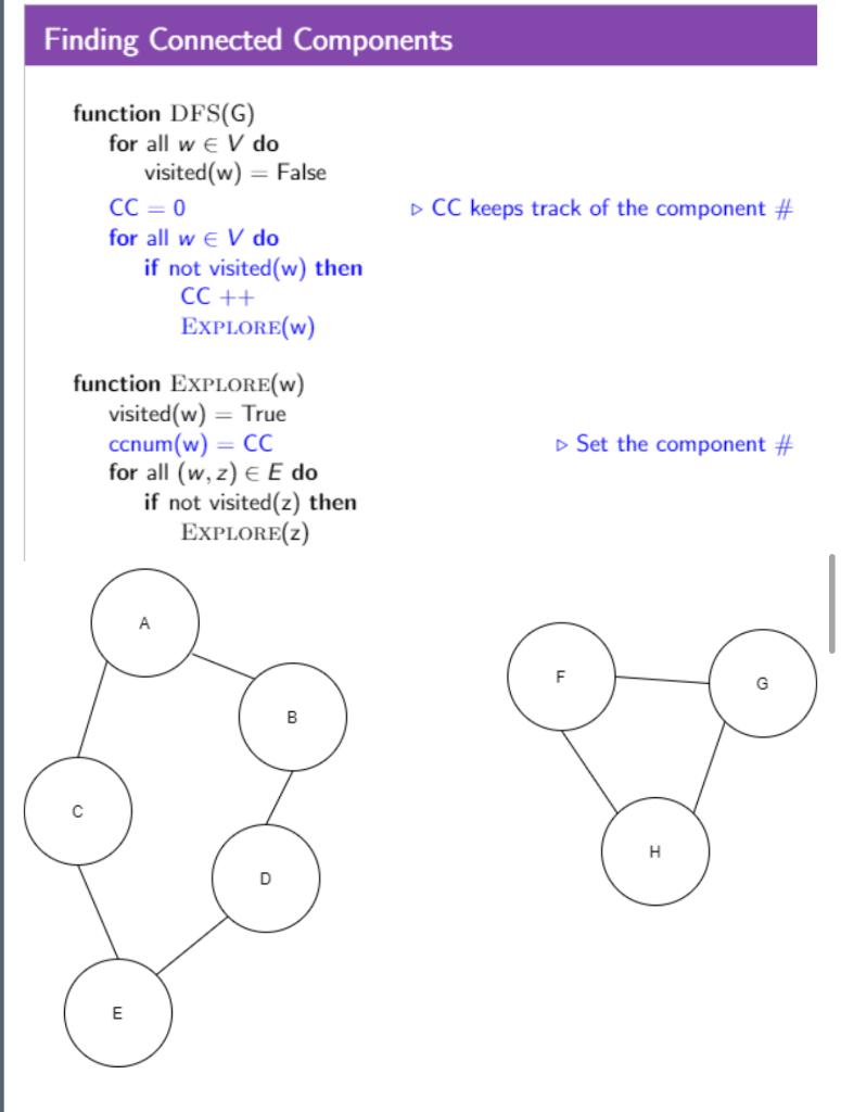
Let's trace the algorithm shown in the image on the sample graph:

1. Initialization: visited array is all false, CC = 0.
2. Outer loop DFS(G):
   • w = A: visited[A] is false. Increment CC to 1. Call EXPLORE(A).
   • EXPLORE(A): Marks A as visited (ccnum(A) = 1). It might explore B next.
   • EXPLORE(B): Marks B as visited (ccnum(B) = 1). It might explore D.
   • ... This process continues until A, B, C, D, E are all visited and marked as part of component 1. The EXPLORE calls then backtrack and finish.
   • w = B: visited[B] is now true. The if condition is false, so we skip.
   • ... The loop skips C, D, and E for the same reason.
   • w = F: visited[F] is false. Increment CC to 2. Call EXPLORE(F).
   • EXPLORE(F): Marks F as visited (ccnum(F) = 2). It explores G and H, marking them as part of component 2.
   • ... The loop skips G and H.
3. End: The loop finishes. The algorithm has correctly identified 2 components and assigned each vertex to one.

The video below walks through this exact process, explaining how to assign a component ID to each node during the traversal.

C++ Implementation and Proof of Correctness

Now let's look at a concrete implementation. The logic is a direct translation of the pseudocode we just discussed. We'll have a main function that iterates through all vertices and a recursive dfs helper function.

The find_comps function in the provided code is the driver. It uses a used vector (our visited array). The comp vector is used to store the nodes of the current component being explored. In many competitive programming problems, you might instead want a persistent array, say component_id[N], that stores the component number for each vertex, just like in the ccnum(w) pseudocode from the image.

A quick exercise for you: How would you modify the provided C++ code to populate a vector<int> component_id of size n instead of just printing the components?

Proof of Correctness

Why does this simple procedure work? We need to be sure that a single DFS call from an unvisited vertex v finds all vertices in its component and no vertices outside of it.

The proof formalizes our intuition.

1. A traversal (DFS or BFS) starting at v can never reach a vertex outside v's connected component, by the very definition of a component (no connecting path exists).
2. The traversal will reach every vertex inside v's component. The proof shows this by induction on the distance (number of edges) from v. It correctly reaches v (distance 0). If it reaches all vertices at distance i, it will also discover their neighbors at distance i+1, thus eventually reaching all vertices in the component.

Complexity Analysis and A Practical Note

Time Complexity: The main loop in find_comps iterates V times. However, the dfs function is only called on a vertex if it hasn't been visited yet. This ensures that each connected component is traversed exactly once. Over all the calls to dfs, each vertex is visited once, and each edge (u, v) is considered twice (once from u's adjacency list and once from v's). Therefore, the total time complexity is $O(V+E)$, which is linear in the size of the graph.

Space Complexity: The space required is dominated by the visited array and the recursion stack for DFS. Both are proportional to the number of vertices, so the space complexity is $O(V)$.

Recursive vs. Iterative DFS:
For competitive programming, it's worth noting a potential pitfall of recursive DFS. If a graph has a very long path (e.g., 1 -> 2 -> 3 -> ... -> 10^5), the recursion depth can become very large, potentially causing a stack overflow error. The cp-algorithms article you read briefly mentions this and shows an iterative version using an explicit std::stack. For most problems, the recursive version is cleaner and sufficient, but it's crucial to be aware of this limitation and the iterative alternative.

Conclusion

In this lesson, you have learned a fundamental graph algorithm that is both simple and efficient. By combining a simple loop with the DFS traversal you already know, you can now systematically partition any undirected graph into its constituent connected components.

Key Takeaways:

• A connected component is a maximal subgraph where every vertex is reachable from every other vertex.
• The algorithm to find all components involves iterating through all vertices and launching a DFS from any vertex that has not yet been visited.
• Each new DFS call from the main loop corresponds to discovering one new component.
• The algorithm is highly efficient, running in $O(V+E)$ time.
• This technique can be used to either count the components or to assign a unique ID to each vertex indicating which component it belongs to.

You've now seen how to use traversals to find shortest paths (BFS) and to identify connected components (DFS). In our next lesson, we will continue augmenting DFS to solve another critical problem: detecting cycles in both undirected and directed graphs.