Building an Evaluation Framework for Machine Learning Models

The Asymmetric Cost of Errors

In classification, we often talk about a model's predictions in terms of a confusion matrix, which categorizes outcomes into four types.

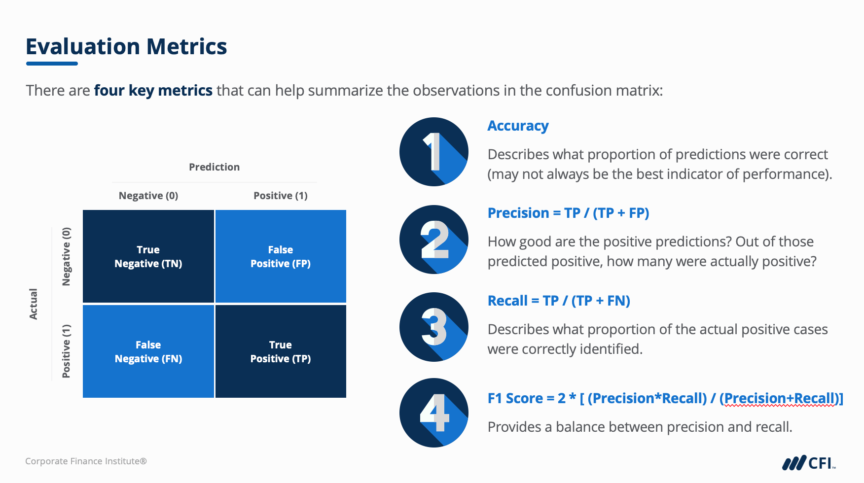
In many machine learning applications, all errors are treated equally. However, in credit risk, the two types of errors have vastly different financial consequences.

• False Positive (FP): The model predicts the applicant is "low risk" (will repay), but they actually default.
  • Business Impact: The financial institution approves a bad loan and likely loses a significant portion of the principal amount, plus any associated collection costs. This is a direct, tangible loss.
• False Negative (FN): The model predicts the applicant is "high risk" (will default), but they would have repaid successfully.
  • Business Impact: The institution rejects a good applicant and loses out on the potential profit from interest payments. This is an opportunity cost.

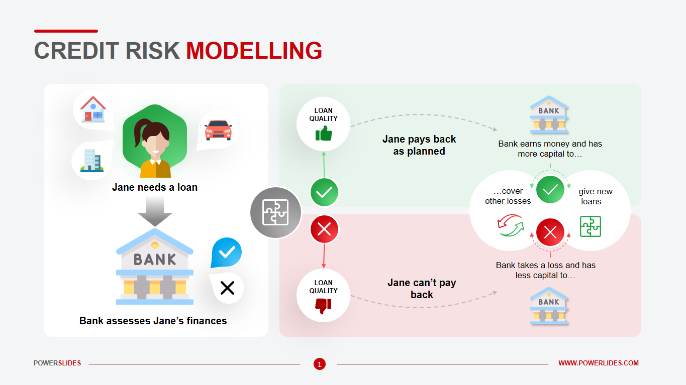
Clearly, the cost of a False Positive is typically an order of magnitude greater than the cost of a False Negative. A model that makes many FP errors could be catastrophic for the business, even if its overall accuracy is high. This is why accuracy is a poor metric for our problem.

Selecting Cost-Sensitive Evaluation Metrics

To build a model that provides business value, our evaluation framework must reflect this cost asymmetry. We need metrics that go beyond a simple count of correct vs. incorrect predictions.

Sensitivity (Recall) and Specificity

A better approach is to evaluate the model's performance on each class independently. Two key metrics for this are Sensitivity and Specificity.

To get a clear definition and see how they are calculated, please watch this excellent explanation from StatQuest.

Let's translate these concepts to our loan default scenario:

• Sensitivity (or Recall): This is the proportion of actual defaulters that the model correctly identifies.
  $\text{Sensitivity (Recall)}=\frac{\text{True Positives}}{\text{True Positives}+\text{False Negatives}}$
  A high sensitivity is crucial for risk management, as it means the model is effective at "catching" high-risk applicants.

• Specificity: This is the proportion of actual good customers (non-defaulters) that the model correctly identifies.
  $\text{Specificity}=\frac{\text{True Negatives}}{\text{True Negatives}+\text{False Positives}}$
  A high specificity is important for business growth, ensuring that creditworthy applicants are not being unnecessarily rejected.

As the video explained, there is often a trade-off. A model that is very aggressive in flagging potential defaults (high sensitivity) may inadvertently reject more good customers (lower specificity). The right balance depends on the institution's risk appetite and business strategy.

Expected Monetary Loss (EML)

While Sensitivity and Specificity are vast improvements over accuracy, they still don't speak the primary language of business: money. The most effective way to evaluate a credit risk model is to quantify its financial impact directly. This is where Expected Monetary Loss (EML) comes in.

The following article provides a superb, business-focused explanation of EML and its importance.

The key formula is:
$EML=\frac{(\text{FP}\times {\text{Cost}}_{\text{FP}})+(\text{FN}\times {\text{Cost}}_{\text{FN}})}{\text{Total Applicants}}$

Where:

• ${\text{Cost}}_{\text{FP}}$ is the average financial loss from approving a bad loan.
• ${\text{Cost}}_{\text{FN}}$ is the average opportunity cost from rejecting a good loan.

The scenario comparing the two banks is powerful: the bank whose model had slightly lower "statistical" performance (like AUC) but was optimized to reduce EML saved millions. This is a core principle of applied data science: the best model is the one that delivers the most business value, not necessarily the one with the highest score on a generic metric.

For our project, we will define Cost_FP and Cost_FN with our business stakeholders and use EML as our primary metric for model selection and tuning. This ensures our technical work remains perfectly aligned with the financial objectives of the business.

Assessing Dataset Suitability

Before we can build and evaluate a model, we must first ensure our data is fit for purpose. An evaluation framework is useless without a valid dataset.

The following technical guide, written for financial institutions, details the practical steps for preparing data for a credit scoring project. We'll focus on two critical aspects.

Based on this reading, here are the key considerations for assessing our dataset:

1. Clarity of the Target Variable ("Define 'Bad'"):
   As we decided in the last lesson, the definition of default (e.g., 90 days past due, or PAR90) is a business decision. This definition must be applied consistently to our historical data to create the ground truth for our model. The guide notes this definition directly impacts how many "bad" examples we will have in our dataset. A more lenient definition (e.g., PAR90) will result in fewer "bads" than a stricter one (e.g., PAR30).

2. Sufficient Number of "Bads":
   Credit default is a rare event, leading to a class imbalance (many more "good" loans than "bad" ones). The guide suggests a rule of thumb: you need at least 500-1500 "bad" examples to build a statistically significant model. If our dataset doesn't meet this threshold, our model's performance on the minority class will be unreliable.

3. Appropriate Sampling Window:
   The data must be both relevant and mature.

   • Relevance: The data should be recent enough to reflect the current economic climate and customer behavior. A model trained on data from 10 years ago may not perform well today.
   • Maturity: The loans in our training sample must have been active long enough for their final outcome to be known. For example, if our performance window is 24 months, we cannot include loans that were issued only 6 months ago, as we don't yet know if they will default within the observation period.

Conclusion

In this lesson, we constructed a professional evaluation framework tailored to the business realities of credit risk. We moved beyond generic metrics to those that capture the asymmetric costs of errors and translate directly to financial impact.

Key Takeaways:

• Asymmetric Costs: In loan default prediction, False Positives (approving a defaulter) are far more costly than False Negatives (rejecting a good applicant). Standard accuracy is therefore a misleading metric.
• Cost-Sensitive Metrics: Our evaluation framework must prioritize metrics that reflect business impact. We will use Sensitivity (Recall) to ensure we effectively identify defaulters and Specificity to ensure we don't turn away too much good business.
• Business-Centric Evaluation: The ultimate metric for model selection will be Expected Monetary Loss (EML), which quantifies the model's financial performance per applicant.
• Dataset Suitability: A reliable model can only be built on suitable data. This requires a clear and consistently applied definition of "default," a sufficient number of default examples, and a carefully chosen sampling window that balances data recency with outcome maturity.

Next Steps:

With our project framed and our evaluation criteria set, we are ready to begin the hands-on work. In the next module, we will dive into the data itself. The first lesson, "Strategic Data Preparation for Credit Risk," will focus on developing a strategy for handling the practical challenges of a real-world dataset, including missing values, outliers, and the class imbalance we identified today.