Introduction
Welcome back to our project. In the last lesson, we designed a robust data preparation strategy to handle missing values, outliers, and the critical issue of class imbalance. We established that these are not just procedural steps, but strategic decisions that form the foundation of a reliable credit risk model.
Today, we build on that foundation by moving into one of the most creative and impactful stages of the modeling process: feature engineering and selection. Raw data rarely contains all the information needed for a high-performing model. A significant part of a data scientist's role is to transform existing data and create new, more predictive features. We will explore how to craft domain-specific features for credit risk, prepare them for modeling through encoding and scaling, and finally, select the most powerful subset of features to build our model.
This lesson directly addresses the learning outcome: Engineer and select domain-specific features for credit risk, justifying choices for encoding and scaling in preparation for modeling.
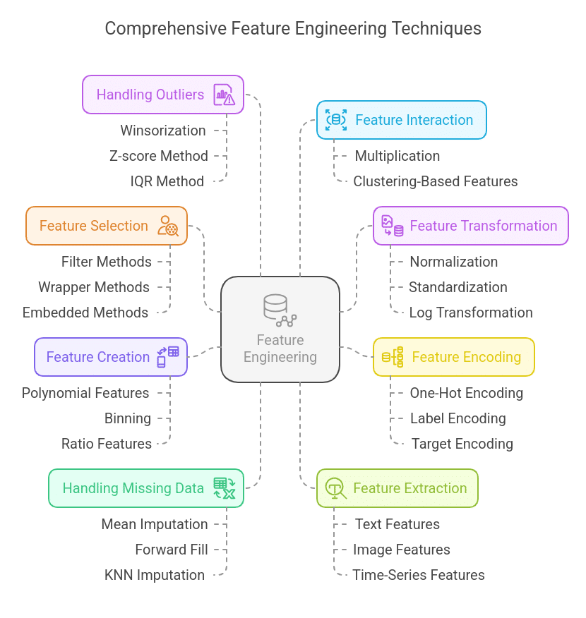
1. Feature Engineering: Creating Predictive Signals
Feature engineering is the art and science of creating new input variables (features) from your raw data. For credit risk, this often involves combining existing features to create ratios and interaction terms that better represent a borrower's financial health.
Creating Interaction and Ratio Features
A single feature, like annual_income, tells part of the story. But its predictive power increases dramatically when combined with other features. For example, a high income is less meaningful if the person also has massive debt. This is where interaction and ratio features come in.
Let's watch a section of a tutorial that explains this concept with clear, credit-risk-specific examples.
Credit Risk Modeling (PD/LGD/EAD): Feature Engineering (Part 3)
This video explains how to create new 'interaction features' by combining existing variables to capture more complex relationships.
Watch the segment from 36:02 to 46:13. Pay close attention to the logic behind creating features like income * age and FICO_score * loan_term. The key idea is that the combination of features can be more predictive than the sum of their parts.
As the video illustrates, creating interaction terms helps the model capture nuanced patterns. In our loan default project, some of the most powerful features are ratios that contextualize financial information. For instance:
- Debt-to-Income Ratio (DTI):
total_debt / annual_income. This is a classic measure of a borrower's ability to manage their payments. A high DTI is a significant red flag. - Credit Utilization Ratio:
total_credit_used / total_credit_limit. This shows how much of their available credit a person is using. High utilization can indicate financial distress. - Loan Payment to Income Ratio:
loan_installment_amount / monthly_income. This assesses the affordability of the specific loan being applied for in the context of the borrower's income. - Loan Amount to Income Ratio:
loan_amount / annual_income. This measures the size of the loan relative to the borrower's annual earnings.
Creating these domain-specific features is a hallmark of professional data science in finance. They transform raw numbers into economically meaningful indicators of risk that directly improve model performance.
2. Feature Transformation and Preparation
Once we have our set of raw and engineered features, we need to prepare them for our machine learning models. This involves two main steps: encoding categorical variables and scaling numerical variables.
Encoding Categorical Variables
Machine learning algorithms require numerical input. Therefore, we must convert non-numerical, categorical features (like loan_purpose or home_ownership) into a numerical format.
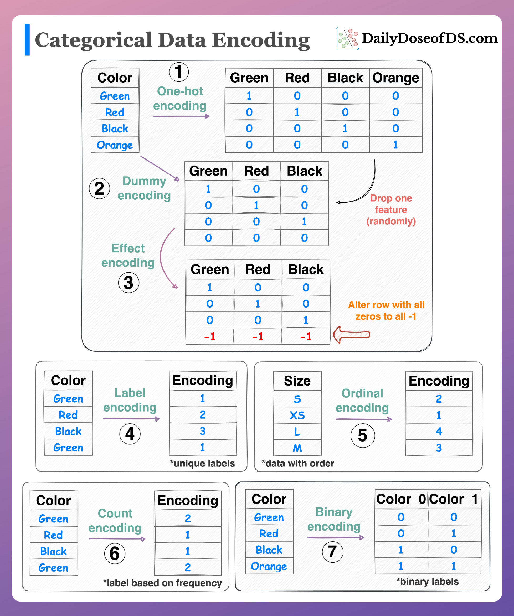
Here are the primary strategies and their trade-offs:
-
One-Hot Encoding: This method converts a categorical feature into multiple new binary (0/1) columns, one for each unique category.
- Pros: It doesn't impose any artificial order on the categories, which is good for nominal variables (where categories have no inherent rank).
- Cons: If a feature has many categories (e.g., 'City'), it can lead to a massive increase in the number of features, known as the "curse of dimensionality."
-
Label Encoding: This assigns a unique integer to each category (e.g., 'A'=0, 'B'=1, 'C'=2).
- Pros: Simple and doesn't increase the number of features.
- Cons: It creates an artificial ordinal relationship (e.g., C > B > A), which can mislead models unless the feature is truly ordinal (e.g., 'low', 'medium', 'high').
-
Target Encoding (or Mean Encoding): This is a more advanced technique where each category is replaced by the average value of the target variable for that category. For example, if 8% of applicants with
loan_purpose = 'car'default, the 'car' category would be encoded as 0.08.- Pros: It's very powerful as it directly uses information from the target to create a predictive feature. It's also memory-efficient.
- Cons: It's highly prone to overfitting and data leakage. To use it correctly, you must calculate the encodings on a training set and then apply them to a separate validation/test set.
Let's hear from an industry expert on which methods are preferred in a real-world financial services company.
Machine Learning in Financial Credit Risk Assessment - Data Science Festival
The data science team at Zopa, a UK financial company, discusses their approach to encoding categorical variables for credit risk.
Watch the section from 13:59 to 16:22. Notice their justification for using target-mean encoding over other methods like one-hot encoding, especially for high-cardinality features.
The preference for target encoding at Zopa highlights an important professional practice: choosing techniques that are both powerful and practical for the problem at hand.
Scaling Numerical Variables
Many algorithms, particularly linear models like Logistic Regression and distance-based models like SVM, are sensitive to the scale of the input features. A feature with a large range (e.g., annual_income) can dominate one with a small range (e.g., number_of_children). We use scaling to bring all features to a comparable level.
How to engineer variables that make credit risk models more reliable?
This article provides a clear explanation and Python code for the two most common scaling techniques: normalization and standardization.
Please read sections 1.2 ('Normalization') and 1.3 ('Standardization'). Focus on the difference in their formulas and the resulting distributions (range of [0, 1] for normalization vs. mean of 0 and standard deviation of 1 for standardization).
To summarize the key distinction:
- Standardization (Z-score Scaling): Transforms data to have a mean of 0 and a standard deviation of 1. It's the default choice for many models, including Logistic Regression, because it centers the data and is less sensitive to outliers than normalization.
- Normalization (Min-Max Scaling): Rescales data to a fixed range, usually [0, 1]. It's often used for algorithms like neural networks that expect inputs within this range.
For our project, where we plan to use Logistic Regression as a baseline, Standardization is the appropriate choice for scaling our numerical features.
3. Feature Selection: Finding the Signal in the Noise
In a real-world credit risk project, you might start with hundreds or even thousands of features from various data sources. Using all of them is inefficient and can lead to overfitting. Feature selection is the process of identifying and keeping only the most predictive variables.
Machine Learning in Financial Credit Risk Assessment - Data Science Festival
Let's return to the Zopa video to understand the business and technical motivations for aggressive feature selection.
Watch from 19:50 to 21:30. The speaker explains why reducing the feature count from 3000 to a few dozen is crucial for implementation speed, reliability, and reducing errors.
As you heard, the goals are to make the model:
- Easier to implement and maintain.
- Faster to score new applicants.
- More reliable and robust by reducing dependency on third-party data providers.
A powerful and widely used technique for feature selection in the credit scoring industry is Information Value (IV).
Information Value (IV)
IV is a metric that measures the predictive power of a single feature in relation to the binary target variable (default vs. non-default). It quantifies how well the feature can distinguish between the two outcomes. It's often used with its component, Weight of Evidence (WoE), which measures the "strength" of each category or bin within a feature.
Credit Risk 2: Feature Selection
This article gives an excellent, concise explanation of WoE and IV and their role in credit risk feature selection.
Read the sections 'WOE & IV' and '4. Binning Strategy for Continuous Variables'. Focus on understanding the conceptual meaning of IV and the strategy of binning continuous variables before calculating their IV.
The general workflow for using IV is:
- For categorical features: Calculate the WoE for each category and then the overall IV for the feature.
- For continuous features: First, bin the feature into groups (e.g., using quantile binning). Then, treat the bins as categories and calculate WoE and IV.
We then use a common rule of thumb to interpret the IV scores:
| Information Value (IV) | Predictive Power |
|---|---|
| < 0.02 | Useless |
| 0.02 to 0.1 | Weak |
| 0.1 to 0.3 | Medium |
| 0.3 to 0.5 | Strong |
| > 0.5 | Suspicious |
A score above 0.5 often indicates data leakage (the feature contains information it shouldn't have during training) and requires investigation.
For our project, our strategy will be to calculate the IV for all our engineered features and select those with 'Medium' or 'Strong' predictive power for inclusion in our model. This is a robust, industry-standard filter method that provides a strong and interpretable feature set.
Conclusion
In this lesson, we've developed a comprehensive strategy for the final and most creative phase of data preparation. We've gone beyond simple cleaning to actively sculpting our dataset for maximum predictive performance.
Key Takeaways:
- Feature Engineering: We create new, powerful predictors by combining existing variables into domain-specific ratios and interactions (e.g., Debt-to-Income Ratio).
- Categorical Encoding: We must convert categorical data to numbers. While One-Hot Encoding is common, Target Encoding is a powerful technique used in industry, though it must be handled carefully to prevent overfitting.
- Numerical Scaling: For models like Logistic Regression, we must scale numerical features. Standardization (Z-score) is generally preferred as it centers the data and handles outliers better than normalization.
- Feature Selection: To build an efficient and robust model, we select only the most predictive features. Information Value (IV) is an industry-standard filter method in credit risk for quantifying a feature's predictive power.
Next Steps:
Our data is now fully prepared. We have cleaned it, engineered new signals, and selected the most powerful features. In the next lesson, Comparative Modeling and Selection, we will finally start building models. We'll implement our modeling pipeline, incorporate the SMOTE technique we identified for handling class imbalance, and train and compare a simple baseline model (Logistic Regression) against a more complex one (XGBoost) to select our final champion model.