Big-O Notation: Analyzing Algorithm Complexity

Why Do We Need a Formal Measure for Efficiency?

Before we dive into the "how," let's establish the "why." You might wonder why we don't just measure an algorithm's speed in seconds. The problem is that the time taken to run a program depends on many factors: the CPU speed, the amount of RAM, and even other programs running on the machine. An algorithm might take 2 seconds on an old laptop but only 1 second on a new one. This makes direct time measurement an unreliable, apples-to-oranges comparison.

We need a way to talk about an algorithm's efficiency that is independent of the hardware. This is where Big-O notation comes in. It doesn't measure time in seconds; instead, it describes how the number of operations an algorithm performs scales as the input size grows. It measures the rate of growth of the runtime, not the absolute runtime itself.

To get a clear understanding of this crucial distinction, please watch the first part of the following video from the "take U forward" channel.

What are Time and Space Complexity?

When we analyze an algorithm, we're typically concerned with two resources:

1. Time Complexity: How the runtime of an algorithm grows as the input size (n) increases.
2. Space Complexity: How the amount of memory an algorithm uses grows as the input size (n) increases.

Big-O notation is the mathematical language we use to express both. It provides an upper bound on the growth rate, which is why it's so useful for predicting performance in the worst-case scenario.

For a formal definition, let's turn to a helpful article from DesignGurus.

The Rules of Calculation

Calculating Big-O might seem complex, but it's guided by a few straightforward rules that simplify the process. We're interested in the "big picture" of how an algorithm scales, so we can ignore the details that don't significantly impact its growth curve for large inputs.

The "take U forward" video explains these rules very clearly.

An important note on space complexity: it is generally defined as the sum of input space (the memory used to store the input) and auxiliary space (any extra memory the algorithm needs). In many contexts, especially interviews, "space complexity" refers only to the auxiliary space. It's a good practice to clarify this if ambiguity arises. A crucial rule of thumb in software engineering is to avoid modifying the input data unless explicitly told to. It's better to use extra space (auxiliary space) than to risk corrupting data that might be used elsewhere in the system.

A Tour of Common Complexity Classes

Now, let's explore the most common Big-O complexities, from most efficient to least efficient. Understanding this hierarchy is key to evaluating algorithms.

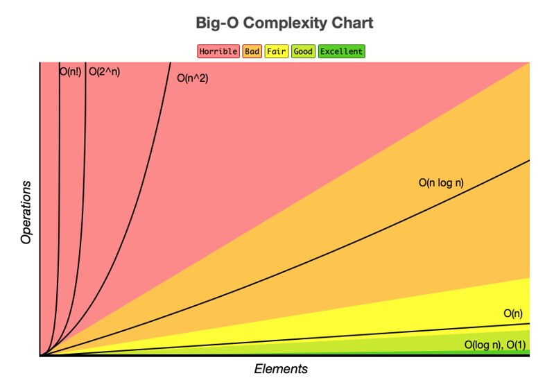
The following video from NeetCode provides a fantastic, practical tour of these complexities with code examples. As you watch, pay attention to how different code structures (loops, nested loops, recursion) map to different Big-O classes.

Let's quickly analyze the time and space complexity of a few key examples from the resources.

1. Linear Search

This algorithm iterates through an array to find an element.

def linear_search(arr, x):
  for i in range(len(arr)):
    if arr[i] == x:
      return i
  return -1

• Time Complexity: $O(n)$. In the worst case, we have to check every single one of the $n$ elements.
• Space Complexity: $O(1)$. We only use a few variables (i, x), and the memory required does not grow with the input array's size.

2. Bubble Sort (Simple version)

This algorithm uses nested loops to sort an array.

def bubble_sort(arr):
  n = len(arr)
  for i in range(n):
    for j in range(0, n - i - 1):
      if arr[j] > arr[j + 1]:
        arr[j], arr[j + 1] = arr[j + 1], arr[j]

• Time Complexity: $O(n^2)$. The outer loop runs $n$ times, and the inner loop runs approximately $n$ times for each outer iteration. This nested structure leads to quadratic complexity.
• Space Complexity: $O(1)$. The sorting is done "in-place," meaning we are modifying the original array and not using any extra space that scales with the input size.

3. Recursive Fibonacci

This is a classic (though inefficient) example of calculating Fibonacci numbers.

def fibonacci(n):
  if n <= 1:
    return n
  else:
    return fibonacci(n - 1) + fibonacci(n - 2)

• Time Complexity: $O(2^n)$. Each call to fibonacci(n) generates two more calls. This creates a recursive tree that grows exponentially.
• Space Complexity: $O(n)$. The space is determined by the maximum depth of the recursion call stack. To calculate fibonacci(n), the call stack can go as deep as n, storing the state for each call.

A Practical Rule of Thumb

In competitive programming and online coding platforms, there's a useful heuristic: a typical server can perform about $10^8$ operations per second. This gives you a concrete way to estimate if your algorithm is fast enough.

• If your input size N is $10^5$, an $O(n^2)$ algorithm would require roughly $(10^5{)}^2=10^{10}$ operations, which is too slow (it would take ~100 seconds).
• An $O(n\log n)$ algorithm would be about $10^5\times {\log }_2(10^5)\approx 10^5\times 17$, which is roughly $1.7\times 10^6$ operations—well within the one-second limit.

This shows why choosing an algorithm with a lower time complexity is not just an academic exercise; it has direct, practical consequences on performance.

Conclusion

You now have the fundamental tools to analyze algorithm performance. Let's summarize the key takeaways:

• Big-O measures scalability, not speed. It describes the rate of growth of an algorithm's time or space requirements as the input size n increases.
• We simplify by focusing on what matters. We analyze the worst-case scenario and drop constants and non-dominant terms to understand the overarching growth trend.
• There is a clear hierarchy of efficiency. Algorithms with complexities like $O(\log n)$ or $O(n)$ are highly efficient and scale well. Those with complexities like $O(n^2)$ are acceptable for small inputs but become slow quickly. Exponential and factorial time complexities are generally impractical for anything but very small inputs.

This cheat sheet provides a great summary of the complexities for common data structure operations and sorting algorithms, which you will encounter throughout this course.

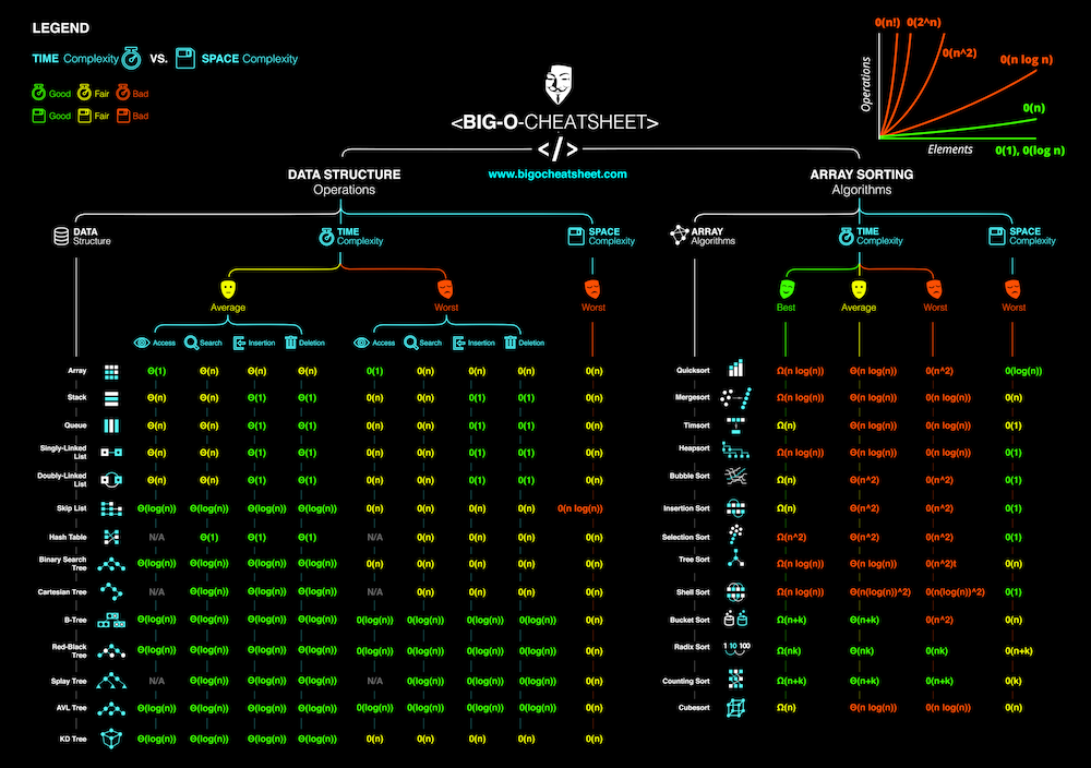
In our next lesson, we will begin applying this knowledge. We will dive into the first group of fundamental data structures—arrays, linked lists, and hash maps—and use Big-O notation to compare their trade-offs for various operations.