Introduction
Hello! In our previous lesson, we explored the significance of the Cramér-Rao Lower Bound (CRLB). You learned that for any unbiased estimator, the CRLB provides an absolute lower limit on its variance, acting as a "gold standard" for efficiency. This is a powerful result, but it relies on knowing the full probability distribution of the data to calculate the Fisher Information.
Today, we shift our focus to a different, yet equally fundamental, theorem of optimality: the Gauss-Markov theorem. This theorem provides a guarantee of optimality within a more restricted class of estimators—specifically, linear and unbiased estimators. Its power lies in requiring weaker assumptions; we only need to know the first two moments (mean and variance) of the error terms, not their entire distribution.
Our goal for this lesson aligns directly with the learning outcome: to prove the Gauss-Markov theorem, which states that the Ordinary Least Squares (OLS) estimator is the Best Linear Unbiased Estimator (BLUE).
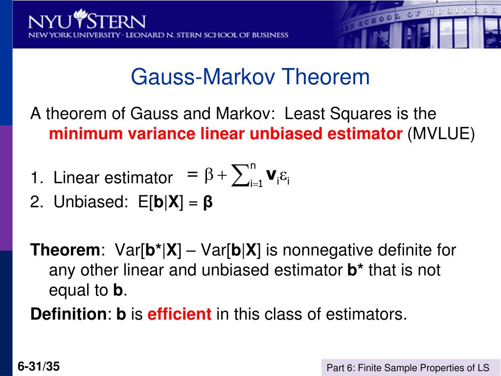
By the end of this lesson, you will have rigorously derived this cornerstone result of linear regression, understanding precisely what "best" means in this context and under which conditions it holds.
1. Setting the Stage: The Linear Model and its Assumptions
Before we can prove the theorem, we must be precise about the model and the "rules of the game"—the assumptions under which the theorem is valid.
Recall the general linear model in matrix form:
where:
- is the vector of observed outcomes.
- is the matrix of predictors (the design matrix).
- is the vector of unknown coefficients we want to estimate.
- is the vector of unobserved random errors.
The OLS estimator for is given by the formula you've seen before, derived from the normal equations:
The Gauss-Markov theorem holds if a specific set of assumptions about this model are true. Please read the following section from StatLect to familiarize yourself with these assumptions.
Gauss Markov theorem - StatLect
This reading clearly lays out the linear regression model and the key assumptions required for the Gauss-Markov theorem in matrix notation.
Please read the section titled 'Assumptions'. Focus on the three numbered points that define the properties of the error term and the design matrix.
To summarize, the Gauss-Markov assumptions are:
-
Zero Mean Error: The expected value of the error term, conditional on the predictors, is zero.
This means that, on average, the model is correctly specified. -
Spherical Errors: The errors are homoscedastic (have constant variance, ) and uncorrelated.
where is the identity matrix. From your mechanical engineering background, you can think of this as assuming the measurement noise has the same magnitude regardless of the system's state and that each measurement's error is independent of the others. -
Full Rank Design Matrix: The matrix has full column rank (). This means there is no perfect multicollinearity among the predictors, ensuring that is well-defined.
Crucially, notice what is not assumed: we have not assumed that the errors follow a Normal distribution. This is a key difference from the assumptions often made when deriving properties of Maximum Likelihood Estimators.
2. Deconstructing BLUE: Linearity and Unbiasedness
The acronym BLUE stands for Best Linear Unbiased Estimator. Let's prove the "L" and "U" parts first.
-
Linear: An estimator is linear if it is a linear function of the observed outcomes . Looking at the OLS formula, , we can see it is the product of a matrix (which is fixed for a given ) and the vector . This is a linear transformation, so is a linear estimator.
-
Unbiased: An estimator is unbiased if its expected value equals the true parameter value. We need to prove .
The following reading provides a concise proof for both of these properties.
Gauss Markov theorem - StatLect
This section provides the formal proof that the OLS estimator is both linear in the outcome variable and an unbiased estimator of the true parameter vector.
Read the section 'OLS is linear and unbiased', paying close attention to the mathematical steps in the 'Proof' box for unbiasedness.
Let's walk through the proof of unbiasedness together, as it's a foundational step:
- Start with the definition of :
- Substitute :
- Distribute the term:
- The first term simplifies, since :
- Now, take the expectation. Since and are fixed (non-random), and using Assumption 1 ():
This completes the proof that is an unbiased estimator of .
3. The Main Event: Proving "Best"
Now we arrive at the heart of the theorem: proving that the OLS estimator is "Best".
What Does "Best" Mean?
In the context of estimators, "best" means having the minimum variance. Since is a vector, its "variance" is a covariance matrix, . For one estimator to be "better" than another estimator , we require that the matrix is positive semi-definite.
This is a generalization of one scalar being greater than or equal to another. It ensures that for any linear combination of the coefficients (e.g., ), the variance of the estimate from OLS is less than or equal to the variance from the alternative estimator.
The Proof Strategy
Our strategy is as follows:
- Define an arbitrary alternative linear unbiased estimator, .
- Derive a condition that this estimator must satisfy to be unbiased.
- Calculate the covariance matrix of .
- Show that this covariance matrix is equal to the covariance matrix of the OLS estimator, , plus a positive semi-definite matrix.
The following video provides an excellent walkthrough of the matrix algebra involved in this proof.
The Gauss-Markov Theorem proof - matrix form - part 3
This video masterfully executes the core of the Gauss-Markov proof. It starts by defining an alternative linear unbiased estimator and then uses matrix algebra to show that its variance can be decomposed into the OLS variance plus a non-negative term.
Watch this video from the beginning to end (it's less than 5 minutes). Follow the algebraic steps closely as the presenter expands the variance expression and uses the unbiasedness condition to simplify it.
Let's formalize the steps from the video with our notation.
Step 1: Define an Alternative Estimator
Let be any other linear estimator. We can write it as a linear function of :
To easily compare it to the OLS estimator, let's define the matrix in terms of the OLS matrix plus some other matrix :
So, our alternative estimator is .
Step 2: Apply the Unbiasedness Condition
We require to be unbiased, i.e., .
For this to equal for any possible , we must have , which implies:
This is a crucial result we will use shortly.
Step 3: Calculate the Covariance of the Alternative Estimator
Now we find the covariance matrix of .
Since is a constant (non-random) term, it does not contribute to the variance. So, we have:
Using the rule and Assumption 2 ():
This is the starting point of the video. As shown, when we multiply this out, we get four terms:
Step 4: Simplify the Expression
- Term 1: Simplifies to . Note that is precisely .
- Term 3: Since from our unbiasedness condition, this term is .
- Term 2: We can rewrite this as . Since , this term is also .
- Term 4: The term remains.
Step 5: The Final Result
Putting it all together, the expression for the variance of our alternative estimator simplifies beautifully:
Therefore,
The matrix is always positive semi-definite. This is because for any non-zero vector , the quadratic form .
This means the variance of any other linear unbiased estimator is equal to the variance of the OLS estimator plus a "non-negative" matrix. This proves that OLS has the minimum variance. For a more detailed textual reference of this final step, you can consult the following resource.
Gauss Markov theorem - StatLect
This resource provides the final step of the proof, showing how the variance of any linear unbiased estimator decomposes into the OLS variance plus a positive semi-definite matrix.
Read the section 'OLS is BLUE'. It formally constructs the alternative estimator and shows that the difference in covariance matrices is positive semi-definite.
Conclusion
Congratulations! You have now walked through the complete proof of the Gauss-Markov theorem. This is a significant result in statistics and econometrics, and understanding its derivation is a mark of a deep theoretical foundation in data science.
Key Takeaways:
- The Meaning of BLUE: The OLS estimator is the Best Linear Unbiased Estimator for the coefficients of a linear model.
- Best: It has the minimum variance among all linear unbiased estimators. This is guaranteed by showing the difference in covariance matrices is positive semi-definite.
- Linear: The estimator is a linear function of the observed data .
- Unbiased: Its expected value is equal to the true parameter vector .
- The Required Assumptions: The theorem relies on the Gauss-Markov assumptions: zero mean errors, homoscedasticity, no error correlation, and no perfect multicollinearity. It does not require the errors to be normally distributed.
- Proof Strategy: The proof hinges on defining an arbitrary linear unbiased estimator and showing its variance equals the OLS variance plus a positive semi-definite matrix (). The unbiasedness condition () is the key that makes the cross-product terms in the variance expansion disappear.
While the CRLB we studied previously gives an absolute bound on variance for any unbiased estimator, the Gauss-Markov theorem provides a powerful guarantee of optimality within the practical and widely-used class of linear estimators, and under less restrictive distributional assumptions.
Preview of the Next Lesson:
We have now explored two major frameworks for estimation: Maximum Likelihood (with its CRLB optimality) and Least Squares (with its Gauss-Markov optimality). Both are part of the "frequentist" school of statistics, which treats parameters as fixed, unknown constants. In the next lesson, we will pivot to a different philosophy: Bayesian Inference. You will learn how to treat parameters as random variables themselves and how to derive estimators like the Minimum Mean Square Error (MMSE) and Maximum A Posteriori (MAP) by combining prior beliefs with observed data.