Sufficient Statistics and the Rao-Blackwell Theorem

Introduction

Welcome to the next lesson on the foundations of statistical inference. In our previous lessons, we've focused on constructing estimators using methods like the Method of Moments. We now turn to a more fundamental question: how do we know if an estimator is good, and more importantly, how can we systematically improve an existing estimator?

This lesson introduces two powerful concepts that form the bedrock of modern estimation theory. First, we will define a sufficient statistic, which you can think of as the ultimate "lossless compression" of your data with respect to a specific parameter. It's a function of the data that captures all the relevant information the sample provides about an unknown parameter, discarding everything else.

Second, we will use this concept to understand and prove the Rao-Blackwell Theorem. This theorem provides a remarkable recipe: take any unbiased estimator (even a poor one), condition it on a sufficient statistic, and you will produce a new estimator that is also unbiased and has a variance that is less than or equal to the original. It gives us a direct path to better estimators.

This lesson aligns perfectly with your interest in mathematical rigor, as we will formally define these concepts and derive the Rao-Blackwell theorem from first principles.

1. Sufficient Statistics: The Art of Data Distillation

Imagine you have a series of sensor readings from a process in your EV battery testing lab. To estimate a physical parameter, say the average internal resistance, do you need the entire time-series history of every single reading, or is a summary, like the sample mean, enough? The concept of sufficiency formalizes this idea.

A statistic $T (X_{1}, ..., X_{n})$ is sufficient for a parameter $θ$ if it contains all the information in the sample about $θ$ . More formally, the conditional distribution of the data given the statistic, $P (X_{1} = x_{1}, ..., X_{n} = x_{n} ∣ T = t)$ , does not depend on $θ$ . Once you know the value of the sufficient statistic, the original data provides no further insight into the parameter.

To learn the intuitive and formal definitions, let's start with a video.

Sufficient Statistics and the Factorization Theorem

This video from Stats with Brian introduces the concept of a sufficient statistic, distinguishing it from a parameter and explaining its role in summarizing data. It also introduces the key tool for finding sufficient statistics: the Factorization Theorem.

Watch the segment from the beginning to 08:25. Pay close attention to: The intuitive definition of sufficiency ('enough' information). The formal introduction of the Neyman-Fisher Factorization Theorem. The reason why sufficiency is important for methods like Maximum Likelihood Estimation and Bayesian Inference.

The Neyman-Fisher Factorization Theorem

As the video explained, checking the definition of sufficiency directly can be cumbersome. The Neyman-Fisher Factorization Theorem gives us a much more practical method.

A statistic $T (X)$ is sufficient for $θ$ if and only if the joint probability density function (or mass function) of the sample, $L (x; θ)$ , can be factored into two parts:

L (x_{1}, ..., x_{n}; θ) = g (T (x_{1}, ..., x_{n}), θ) \cdot h (x_{1}, ..., x_{n})

$g (T (x), θ)$ is a function that depends on the data only through the statistic $T (x)$ . This part contains all the interaction between the data and the parameter $θ$ .
$h (x)$ is a function that depends only on the data $x$ and not on the parameter $θ$ .

Let's see this theorem in action and walk through a formal proof.

4. Sufficiency

These lecture notes from Christian Remling provide a rigorous treatment of sufficiency and the Factorization Theorem. We'll use this to solidify the concepts from the video.

Read Section 4.1, 'Sufficient statistics' (pages 38-41). Focus on: Definition 4.1, the formal definition of sufficiency. Theorem 4.2, the Neyman-Fisher Factorization Theorem, and its proof. Examples 4.2 (Poisson) and 4.3 (Chi-squared), which show how to apply the theorem by inspecting the likelihood function.

Let's re-examine the Poisson distribution example from the video using the notation from the PDF.

Suppose $X_{1}, ..., X_{n}$ are i.i.d. Poisson( $θ$ ). The joint probability mass function (the likelihood) is:

L (x; θ) = i = 1 \prod n \frac{e ^{- θ} θ ^{x_{i}}}{x _{i} !} = \frac{e ^{- n θ} θ ^{\sum x_{i}}}{\prod x _{i} !}

We can factor this as:

L (x; θ) = g (T (x), θ) (e^{- n θ} θ^{\sum x_{i}}) \cdot h (x) (\frac{1}{\prod x _{i} !})

Here, we can see that:

$T (X) = \sum_{i = 1}^{n} X_{i}$ is our statistic.
The function $g$ depends on the data only through the sum $\sum x_{i}$ .
The function $h$ does not depend on $θ$ .

Therefore, by the Factorization Theorem, $T (X) = \sum X_{i}$ is a sufficient statistic for $θ$ .

2. The Rao-Blackwell Theorem: Building Better Estimators

Now that we can identify a sufficient statistic, how do we use it? The Rao-Blackwell Theorem gives us a powerful, constructive method to improve estimators.

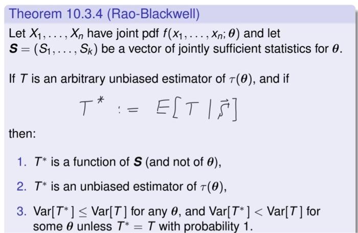
Rao-Blackwell Theorem Statement — This is the formal statement of the Rao-Blackwell Theorem. It provides a method to take an unbiased estimator, T, and use a sufficient statistic, S, to create a new estimator, T*, that is at least as good, if not better.

The theorem tells us that if we have any unbiased estimator $T_{1}$ for $θ$ , we can create a new, improved estimator $T_{2}$ by taking the conditional expectation of $T_{1}$ given a sufficient statistic $Y$ .

$T_{2} = E (T_{1} ∣ Y)$

The theorem guarantees two things about $T_{2}$ :

It remains unbiased: $E [T_{2}] = θ$ .
It has a smaller (or equal) variance: $V a r (T_{2}) \leq V a r (T_{1})$ .

The process of creating $T_{2}$ from $T_{1}$ is often called Rao-Blackwellization.

The following video provides an excellent intuitive explanation of the theorem, how it works, and a sketch of its proof.

The Rao-Blackwell Theorem Explained

This video, also from Stats with Brian, explains the Rao-Blackwell theorem with clear, step-by-step examples. It demonstrates how to start with a 'bad' estimator and systematically improve it.

Please watch the following segments: Introduction (00:00 - 01:12): This sets up the motivation for the theorem. First Example (01:12 - 04:31): This shows how to improve an estimator for the Poisson parameter λ. It perfectly illustrates the process of Rao-Blackwellization. Formal Statement (08:22 - 11:27): This part formally states the theorem and explains its implications for bias and variance, using the Law of Iterated Expectation. Proof Sketch (13:36 - 15:12): This provides a quick but powerful look at the mathematical proof, which uses Jensen's Inequality and the Law of Iterated Expectation.

The Mathematical Proof of the Rao-Blackwell Theorem

You have a strong interest in the mathematical underpinnings, so let's go through the proof with more rigor, as presented in the lecture notes. The proof elegantly combines properties of conditional expectation and the definition of sufficiency.

4. Sufficiency

We will now study the formal proof of the Rao-Blackwell theorem. To do so, we first need to understand the properties of conditional expectation, which is the mathematical engine behind the theorem.

Please read Sections 4.2 ('Conditional expectation') and 4.3 ('The Rao-Blackwell Theorem') on pages 42-47. In Section 4.2, focus on: Proposition 4.3 and its proof, which establishes the Law of Total Expectation: E(E(X|Y)) = EX. Theorem 4.5 and its proof, which establishes the variance inequality: Var(E(X|Y)) <= Var(X). In Section 4.3, carefully follow the proof of Theorem 4.6 (Rao-Blackwell). Notice the critical step where the sufficiency of Y is invoked to ensure the new estimator T2 is indeed a statistic (i.e., independent of θ).

Let's summarize the logic of the proof:
Let $T_{1}$ be an unbiased estimator for $θ$ , and let $Y$ be a sufficient statistic for $θ$ . Define $T_{2} = E (T_{1} ∣ Y)$ .

Is $T_{2}$ a statistic? Yes. The conditional expectation $E (T_{1} ∣ Y)$ is a function of the random variable $Y$ . Because $Y$ is sufficient, the conditional distribution of $T_{1}$ given $Y$ does not depend on $θ$ . Therefore, the resulting expectation, $T_{2}$ , is a function of the data only and does not depend on the unknown $θ$ . This is a crucial point that is often missed.
Is $T_{2}$ unbiased? Yes. By the Law of Total Expectation (or iterated expectations):
$E [T_{2}] = E [E (T_{1} ∣ Y)] = E [T_{1}]$
Since $T_{1}$ is unbiased ( $E [T_{1}] = θ$ ), then $E [T_{2}] = θ$ , so $T_{2}$ is also unbiased.
Is the variance reduced? Yes. By the Law of Total Variance (as shown in the proof of Theorem 4.5 in the reading):
$V a r (T_{1}) = V a r (E (T_{1} ∣ Y)) + E [V a r (T_{1} ∣ Y)]$
Substituting $T_{2} = E (T_{1} ∣ Y)$ , we get:
$V a r (T_{1}) = V a r (T_{2}) + E [V a r (T_{1} ∣ Y)]$
Since variance is always non-negative, $E [V a r (T_{1} ∣ Y)] \geq 0$ , which implies:
$V a r (T_{1}) \geq V a r (T_{2})$

The variance of the new estimator is less than or equal to the variance of the original.

3. Rao-Blackwellization in Action

Let's walk through another complete example to see how this powerful theorem is applied.

Rao-Blackwell Theorem and Example — This example illustrates the complete process for i.i.d. Exponential random variables. We start with an unbiased estimator T=X1, identify a sufficient statistic S=X1+X2, and then use conditional expectation to find the improved estimator T*.

Let's apply this to a sample $X_{1}, ..., X_{n}$ from a Uniform $U (0, θ)$ distribution.

Find a simple unbiased estimator. Let's try $T_{1} = 2 X_{1}$ . Since $E [X_{1}] = θ /2$ , we have $E [T_{1}] = E [2 X_{1}] = 2 E [X_{1}] = 2 (θ /2) = θ$ . So, $T_{1}$ is unbiased, although it seems wasteful as it ignores all data points except the first.
Find a sufficient statistic. The joint PDF is: $L (x; θ) = i = 1 \prod n \frac{1}{θ} I (0 \leq x_{i} \leq θ) = \frac{1}{θ ^{n}} I (x_{(n)} \leq θ) I (x_{(1)} \geq 0)$ where $x_{(n)} = max (x_{i})$ and $x_{(1)} = min (x_{i})$ . We can factor this as: $L (x; θ) = g (T (x), θ) \frac{1}{θ ^{n}} I (x_{(n)} \leq θ) \cdot h (x) I (x_{(1)} \geq 0)$ Thus, $Y = X_{(n)} = max (X_{1}, ..., X_{n})$ is a sufficient statistic.
Apply Rao-Blackwell. We need to compute $T_{2} = E [T_{1} ∣ Y] = E [2 X_{1} ∣ X_{(n)} = y]$ . As derived in the video (LINK at 11:27) and the PDF notes (LINK, Example 4.7), this calculation yields: $T_{2} = \frac{n + 1}{n} Y = \frac{n + 1}{n} X_{(n)}$

This is a much more robust estimator, as it depends on all the data (through the maximum value) and, as proven by the theorem, has a smaller variance than our initial estimator $2 X_{1}$ .

Conclusion

In this lesson, we explored the theoretical foundation for improving statistical estimators. We established that an optimal summary of data for a parameter is its sufficient statistic, and we learned how to find it using the Neyman-Fisher Factorization Theorem. We then proved the Rao-Blackwell Theorem, which provides a concrete procedure to transform any unbiased estimator into a new, superior one by conditioning on this sufficient statistic.

Key Takeaways:

A sufficient statistic is a function of the data that captures all the information a sample has to offer about a parameter.
The Neyman-Fisher Factorization Theorem is the primary tool for identifying sufficient statistics by separating the likelihood function into a parameter-dependent part and a data-dependent part.
The Rao-Blackwell Theorem gives a method to improve any unbiased estimator $T_{1}$ by creating a new estimator $T_{2} = E (T_{1} ∣ Y)$ , where $Y$ is a sufficient statistic.
The improved estimator $T_{2}$ is guaranteed to be unbiased and have variance less than or equal to that of $T_{1}$ .

This process demonstrates a deep principle in statistics: estimators that are functions of sufficient statistics are generally preferable. This leads to the concept of the Minimum Variance Unbiased Estimator (MVUE), which is often found by Rao-Blackwellizing a simple estimator.

Self-Test

Consider a random sample of size $n$ , $X_{1}, ..., X_{n}$ , from a Bernoulli( $p$ ) distribution, where $p$ is the unknown probability of success.

Consider the estimator $p^_{1} = X_{1}$ . Show that it is an unbiased estimator for $p$ .
Show that $T = \sum_{i = 1}^{n} X_{i}$ (the total number of successes) is a sufficient statistic for $p$ .
Apply the Rao-Blackwell theorem to find the improved estimator $p^_{2} = E [p^_{1} ∣ T]$ .
- Hint: By symmetry, $E [X_{1} ∣ T = t] = E [X_{2} ∣ T = t] = ... = E [X_{n} ∣ T = t]$ . What is $E [T ∣ T = t]$ ? Use this to find $E [X_{i} ∣ T = t]$ .

Preview of the Next Lesson:

We now have a powerful tool for improving estimators. But what if we want to find a good estimator from scratch, without starting from a "bad" one? In the next lesson, we will explore Maximum Likelihood Estimation (MLE). This is arguably the most important method of parameter estimation in all of statistics. We will see that MLEs are often functions of sufficient statistics and have desirable properties like asymptotic efficiency. We will derive the MLEs for several distributions and prove the famous result connecting MLE to Ordinary Least Squares (OLS) in linear regression.

Recommended resources