Introduction
In our last lesson, we established a framework for evaluating estimators based on their bias, variance, and consistency. We can now answer the question, "Is this a good estimator?" However, a more fundamental question remains: "How do we find an estimator in the first place?"
This lesson addresses that question by introducing three foundational philosophies for constructing estimators from data. Each method provides a different "recipe" for turning a sample of data into an estimate of an unknown population parameter. We will explore:
- Method of Moments (MoM): An intuitive approach based on matching the characteristics of our sample to the theoretical characteristics of the population.
- Maximum Likelihood Estimation (MLE): A powerful and widely-used method that reframes estimation as an optimization problem: which parameter value makes our observed data the most probable?
- Bayesian Estimation: A paradigm shift where parameters themselves are treated as random variables, and we use data to update our prior beliefs about them into a full posterior probability distribution.
By the end of this lesson, you will understand the purpose and core principles of each of these cornerstone estimation techniques, setting the stage for the detailed derivations and applications that will follow.
1. Method of Moments (MoM): Matching Sample to Theory
The Method of Moments is perhaps the most straightforward way to devise an estimator. The core idea is simple and intuitive: we assume that the moments calculated from our sample should be good approximations of the theoretical moments of the population's underlying distribution.
A population moment is a theoretical property of a distribution. The k-th population moment is defined as . These moments are often functions of the distribution's unknown parameters, .
A sample moment is a value we can compute from our data. The k-th sample moment is .
The MoM strategy is to:
- Express the first few population moments () in terms of the unknown parameters ().
- Set these theoretical expressions equal to their corresponding sample moments ().
- Solve the resulting system of equations for the unknown parameters.
The following video provides an excellent, clear introduction to this idea and works through two key examples.
Method of Moments to Fit Distributions from Data
This video from Steve Brunton's 'Data Driven Science and Engineering' series explains the principle behind the Method of Moments and demonstrates how to apply it to estimate the parameters of a Poisson and a Normal distribution.
Watch the entire video (up to 11:02). Pay close attention to how he connects the theoretical moments (E[X], E[X²]) to the sample moments (x̄, sample second moment) to solve for the unknown parameters.
As the video demonstrated, for a normal distribution , we have two parameters, so we need two moments:
- First moment: . We set this equal to the first sample moment, . This immediately gives us our estimator: .
- Second moment: . We set this equal to the second sample moment, .
Solving for and substituting gives:
The following reading provides a more formal definition and discusses the pros and cons of this method.
STAT 713 MATHEMATICAL STATISTICS II
These formal lecture notes from a mathematical statistics course provide a concise, rigorous definition of the Method of Moments strategy.
Please read Section 7.2.1, 'Method of moments' (pages 26-28). Note the formal strategy and the 'Remarks' at the end, which summarize the practical view of MoM estimators.
Purpose and Summary of MoM:
- Purpose: To provide a quick, simple, and intuitive method for finding parameter estimates.
- Pros: Easy to understand and apply. Estimators are often consistent.
- Cons: Can be less efficient (higher variance) than other methods. Sometimes, the estimates can be nonsensical (e.g., a negative estimate for a variance parameter). It's often considered a "quick and dirty" starting point.
2. Maximum Likelihood Estimation (MLE): Maximizing Plausibility
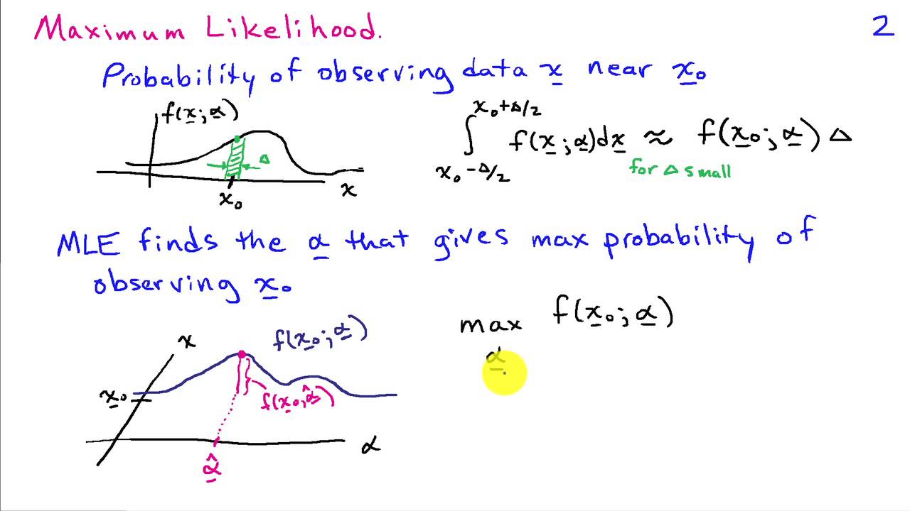
Maximum Likelihood Estimation is a more foundational and powerful method that dominates modern statistics and machine learning. Its guiding principle is: we should choose the parameter values that make our observed data the most probable outcome.
Let's say we have a sample of i.i.d. data points from a distribution . The joint probability of observing this specific dataset is the product of the individual probabilities (or densities):
When we view this expression as a function of the parameter for our fixed, observed data, we call it the likelihood function, .
The MLE is the value of that maximizes this function.
Because maximizing a product of terms can be mathematically cumbersome, we almost always work with the log-likelihood function, . Since the logarithm is a monotonically increasing function, maximizing the log-likelihood is equivalent to maximizing the likelihood itself. The logarithm handily turns the product into a sum:
Finding the MLE then becomes a standard optimization problem, typically solved by taking the derivative with respect to , setting it to zero, and solving.
Let's watch a video that brings this process to life.
Maximum Likelihood Estimation (MLE) with Examples
This video, also from Steve Brunton, provides an excellent walkthrough of Maximum Likelihood Estimation. It explains the construction of the likelihood and log-likelihood functions and derives the MLE for a Poisson distribution step-by-step.
Please watch from 1:01 to 20:21. Focus on: The definition of the likelihood function as a joint probability. The critical step of taking the logarithm to turn the product into a sum. The process of taking the derivative of the log-likelihood and setting it to zero to find the maximizing parameter.
Purpose and Summary of MLE:
- Purpose: To find the parameter values that best explain the observed data from a probabilistic standpoint.
- Pros: Deeply principled, applicable to almost any model. MLEs possess excellent large-sample properties: they are typically consistent, asymptotically unbiased, and have the lowest possible variance among a wide class of estimators.
- Cons: Can be more mathematically involved than MoM. For complex models, the optimization may need to be done numerically.
3. Bayesian Estimation: Updating Beliefs
The Bayesian approach represents a fundamental philosophical shift. In both MoM and MLE (known as frequentist methods), the parameter is considered a fixed, unknown constant. Our goal is to find a single best guess, or point estimate, for it.
In Bayesian inference, the parameter is itself considered a random variable. We begin with a prior distribution, , which represents our beliefs about before seeing any data. We then use the observed data to update our beliefs, resulting in a posterior distribution, .
This update is performed using Bayes' Rule:
Since the denominator, , does not depend on , it acts as a normalization constant. We can therefore state the core of Bayesian inference as:
Unlike MoM and MLE, the result of a Bayesian estimation is not a single point but an entire probability distribution for the parameter. This distribution quantifies our uncertainty about after observing the data. From this posterior, we can compute a point estimate if needed (e.g., the mean, median, or mode of the posterior), but we also get a measure of confidence (e.g., the variance or a credible interval).
To solidify these concepts, the following reading provides a fantastic comparison of all three estimation philosophies.
[PDF] ML, MAP, and Bayesian — The Holy Trinity of Parameter Estimation ...
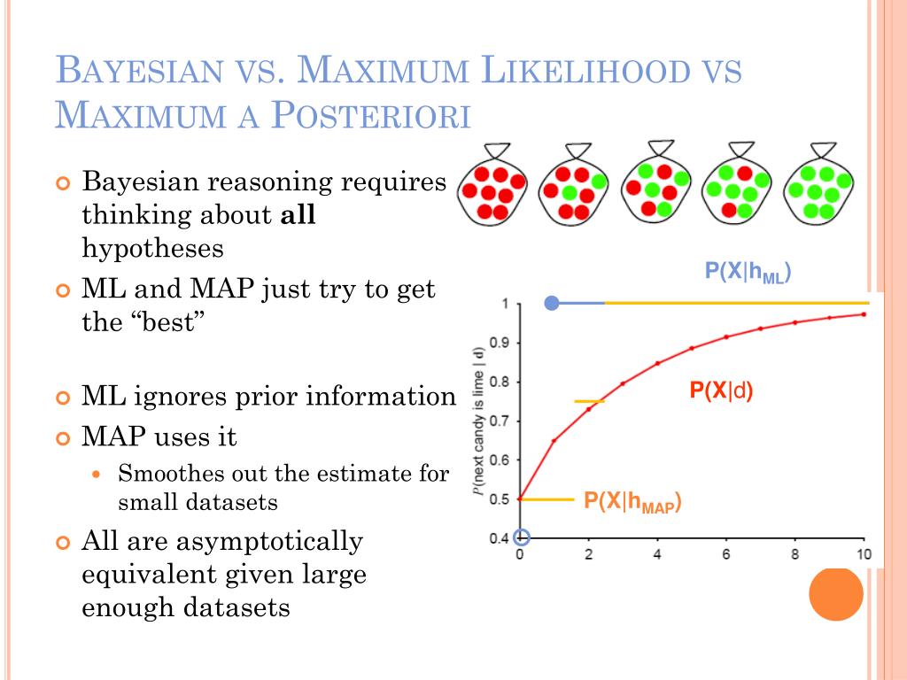
This tutorial by Avi Kak, titled 'ML, MAP, and Bayesian — The Holy Trinity of Parameter Estimation,' offers a clear, side-by-side comparison of these methods. It explains the conceptual differences and mathematical formulations.
Please read the introduction and the sections on ML, MAP, and Bayesian estimation (pages 4 to 27). Pay special attention to: How ML estimation only uses the likelihood prob(X|Θ). How MAP estimation introduces the prior prob(Θ) but still provides a single point estimate (argmax). How full Bayesian estimation calculates the entire posterior distribution prob(Θ|X).
Purpose and Summary of Bayesian Estimation:
- Purpose: To formally update prior beliefs about parameters using observed data, yielding a full probability distribution that quantifies our posterior uncertainty.
- Pros: Provides a complete distributional description of the parameter. Allows for the formal incorporation of prior knowledge, which can be very powerful with small datasets.
- Cons: Can be computationally intensive, as it may require complex integration to find the normalization constant. The choice of prior can sometimes be subjective.
Conclusion
We have now surveyed the three principal methods for constructing estimators. They represent different philosophical approaches to the same fundamental problem: learning from data.
Key Takeaways:
| Method | Core Principle | Output | Role of Prior Beliefs |
|---|---|---|---|
| Method of Moments | Match sample moments to population moments. | Point Estimate | Not used. |
| Max. Likelihood | Find parameters that maximize data likelihood. | Point Estimate | Not used. |
| Bayesian Estimation | Use data to update a prior belief distribution into a posterior distribution. | Full Distribution | Essential component. |
Understanding these three approaches is crucial. While MLE is arguably the most common technique in frequentist statistics and machine learning, the principles of MoM are valuable for their simplicity, and the Bayesian framework is essential for modern applications involving uncertainty quantification.
Preview of the Next Lesson:
Now that we understand the what and why of these methods, we can focus on the how. In the next lesson, we will get our hands dirty with the mathematics of Maximum Likelihood Estimation. We will perform detailed derivations of the MLEs for several common distributions, including the Normal, Exponential, and Poisson. We will also derive the Ordinary Least Squares (OLS) estimator for linear regression and discover its deep connection to MLE, fulfilling your request for rigorous mathematical proofs and connections between concepts.