Visualizing Probability: A Geometric Approach

Introduction

In our last lesson, we explored covariance and correlation, quantifying how random variables move together. We even touched upon a geometric view, seeing correlation as the angle between vectors. Today, we will formalize and expand this geometric intuition to fully describe the relationship between multiple random variables.

This lesson addresses a fundamental question: If we know the probability distribution of variable $X$ and the distribution of variable $Y$, do we know everything about the system $(X,Y)$? As we will see, the answer is no. We need a more comprehensive tool: the joint probability distribution.

Our goal is to construct intuitive, geometric explanations for the three core concepts that govern multiple random variables:

• Joint distributions: A complete picture of the probabilistic landscape.
• Marginal distributions: The individual distributions of each variable, derived from the joint picture.
• Conditional distributions: The distribution of one variable, given that we know the value of another.

This visual understanding is invaluable. It transforms abstract formulas into concrete operations like projecting shadows and taking slices, which resonates well with a background in engineering and physics.

1. Why Individual Distributions Aren't Enough

Imagine you have two projections of a 3D object, one from the front and one from the side. Do you know the exact shape of the original object? Not necessarily. Multiple different 3D objects can cast the same two shadows.

To see this principle in probability, let's start with a resource that provides a wonderful non-mathematical analogy.

This idea is central. The joint distribution captures the complete structure, including the dependencies that are invisible in the individual, or marginal, distributions.

2. The Joint Distribution: A Geometric Landscape

For two continuous random variables $X$ and $Y$, their joint probability density function (PDF), $f(x,y)$, can be visualized as a surface or a landscape over the $x,y$-plane.

• The height of the surface at a point $(x,y)$ corresponds to the probability density at that point.
• The total volume under this entire surface must equal 1.
• The probability that a measurement $(X,Y)$ falls into a specific region $A$ on the plane is the volume under the surface above that region.

Let's watch a short video that introduces this concept using the example of a two-dimensional Gaussian distribution, a shape you'll encounter frequently in data science.

3. Marginal Distributions: Projecting the Shadows

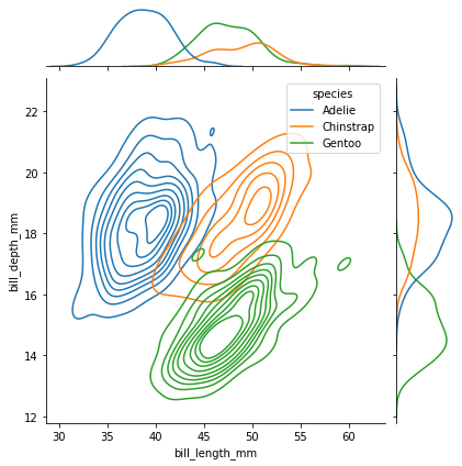
If the joint PDF is a 3D landscape, the marginal PDF of a single variable is its 2D "shadow" projected onto one of the axes.

Imagine the sun is directly overhead. The shadow cast by the probability landscape onto the $x,z$-plane gives you the marginal distribution of $X$, $f_X(x)$. To get the shadow's shape, you effectively "squash" the 3D landscape flat by summing up all the probability density along the $y$-direction for each value of $x$.

Mathematically, this "squashing" is integration. To find the marginal density of $X$ at a point $x$, we integrate the joint density $f(x,y)$ over all possible values of $y$:
$f_X(x)={\int }_{-\infty }^{\infty }f(x,y)dy$
Similarly, for the marginal density of $Y$:
$f_Y(y)={\int }_{-\infty }^{\infty }f(x,y)dx$

This is exactly what is shown in the 3D bar chart above and in the penguin dataset visualization below.

To see the mechanics of this derivation, let's work through a classic example: finding the marginal distributions for a point chosen uniformly from a disk.

As you saw, even though the joint distribution is uniform, the marginal distributions are not. This reinforces the idea from the start of the lesson: the whole is more than the sum of its parts.

4. Conditional Distributions: Taking a Slice

We now move from projection to slicing. A conditional PDF, $f_{Y|X}(y|x)$, answers the question: "Given that I know $X$ is exactly equal to some value $x_0$, what is the new probability distribution for $Y$?"

Geometrically, this is equivalent to taking a thin, vertical slice of our 3D probability landscape at $x=x_0$.

This slice, represented by the curve $f(x_0,y)$, traces the shape of the conditional distribution. However, the area under this curve is not 1, so it's not a valid PDF on its own. The area under this slice is, by definition, the marginal density $f_X(x_0)$.

To turn the slice into a valid PDF, we must normalize it by dividing by its own area. This gives us the fundamental formula for conditional probability:

$f_{Y|X}(y|x)=\frac{f(x,y)}{f_X(x)}=\frac{\text{Joint Distribution}}{\text{Marginal Distribution}}$

The resource below provides excellent visuals for this concept.

Now, let's return to the uniform-on-a-disk example to see how a conditional PDF is derived mathematically.

5. Independence Revisited

The concepts of joint, marginal, and conditional distributions give us a powerful geometric way to understand independence. Two variables $X$ and $Y$ are independent if learning the value of one tells you nothing new about the other.

• In our slicing analogy, this means that the shape of the conditional slice $f_{Y|X}(y|x)$ does not change as you move the slice along the x-axis.
• This implies that the conditional distribution is the same as the marginal distribution: $f_{Y|X}(y|x)=f_Y(y)$.
• Substituting this into the definition of the conditional PDF gives us the famous factorization rule for independence: $f(x,y)=f_X(x)f_Y(y)$. The joint distribution separates into a product of the marginals.

Geometrically, the 2D contours of an independent joint distribution will be aligned with the coordinate axes (like a circle or an axis-aligned ellipse), as seen in the final plot of the "Joint probability distributions – Statistical inference" reading. If the variables are correlated, the contours will be tilted, indicating that the conditional distribution of $Y$ shifts as $X$ changes.

Conclusion

In this lesson, we developed a powerful geometric framework for understanding multivariate probability.

Key Takeaways:

• Joint, marginal, and conditional distributions are the essential tools for describing systems with multiple random variables.
• A joint PDF, $f(x,y)$, can be visualized as a 3D probability landscape.
• A marginal PDF, $f_X(x)$, is a 2D projection (or "shadow") of that landscape, obtained by integrating out the other variable.
• A conditional PDF, $f_{Y|X}(y|x)$, is a normalized 1D slice through the landscape at a fixed value of the conditioning variable.
• Independence has a clear geometric meaning: the shape of the conditional slices does not change as you move them.

Preview of the Next Lesson:
We are now equipped to tackle two of the most important theorems in all of statistics: the Law of Large Numbers (WLLN) and the Central Limit Theorem (CLT). These theorems describe the behavior of sums and averages of many random variables. Our understanding of joint distributions and independence will be a crucial prerequisite, as these theorems typically apply to collections of independent and identically distributed (i.i.d.) random variables. We will start by formally deriving the WLLN using Chebyshev's inequality.