Titanic Data Preparation: A Project-Based Approach

Introduction

In our previous lessons, we've built a solid foundation by mastering NumPy, Pandas, Matplotlib, and, most recently, the core API of Scikit-learn. You've learned how these tools work in isolation. Now, it's time to bring them all together.

This lesson is our first capstone project. We will take on the classic Titanic survival prediction problem, applying everything we've learned to a real-world dataset. Our goal is not yet to build a predictive model, but to perform the crucial preliminary steps that every data scientist must master:

• Loading the data into a workable format.
• Inspecting it to understand its structure and content.
• Cleaning it by handling missing values and irrelevant information.
• Visualizing it to uncover patterns and relationships.

This process, known as Exploratory Data Analysis (EDA), is the heart of data science. The insights we gather here are what inform the modeling choices we'll make later in the course. By the end of this lesson, you will have a clean, prepared dataset, ready for the machine learning algorithms we will study in future modules.

Let's look at the kind of analysis we'll be able to produce.

1. Setting the Stage: The Project Workflow

Our project is to predict survival on the Titanic. Given a passenger's data (like age, class, and sex), can we determine if they were likely to survive the disaster? This is a classic binary classification problem.

Before we write any code, it's essential to have a clear workflow in mind. Let's start by watching a brief overview of the project and importing the libraries we'll need.

As you saw, the standard workflow involves collecting data, processing it, performing analysis, and then training and evaluating a model. This lesson focuses on the first three steps: data collection, processing, and analysis.

2. Loading and Initial Inspection

With our libraries imported, the first practical step is to load the data and get a feel for its structure. We'll load a .csv file into a Pandas DataFrame and use some fundamental DataFrame methods to inspect it.

From this initial inspection, we can draw a few key conclusions:

• The dataset contains 891 entries (passengers) and 12 columns (features).
• The Age, Cabin, and Embarked columns have missing values.
• We have a mix of data types: numerical (Age, Fare), categorical (Sex, Embarked), and text (Name).

3. Data Cleaning: Preparing the Data for Analysis

Raw data is rarely perfect. Our next task is to "clean" it by addressing missing values and converting non-numerical data into a format that a machine learning model can understand.

Handling Missing Values

We have three columns with missing data. We need a strategy for each.

1. Cabin: This column is missing a very large percentage of its values (687 out of 891). Trying to "guess" or impute these values would likely introduce more noise than signal. The best strategy here is to drop the column entirely.
2. Age: This column is missing a significant but manageable number of values (177). Since age is a continuous numerical feature, a common strategy is to replace the missing values with the central tendency of the existing values, such as the mean or median.
3. Embarked: This column is only missing two values. As it's a categorical feature, we can replace the missing entries with the most common port of embarkation (the mode).

Let's see how to implement these strategies in code.

Encoding Categorical Features

Machine learning models are mathematical, which means they work with numbers, not text labels like 'male' or 'female'. We need to convert our categorical text data into a numerical representation. This process is called encoding.

For this project, we'll use a simple mapping:

• Sex: 'male' -> 0, 'female' -> 1
• Embarked: 'S' -> 0, 'C' -> 1, 'Q' -> 2

4. Visualization and Exploratory Analysis

Now that our data is clean, we can start the most exciting part of EDA: asking questions and searching for answers through visualization. Good visualizations can reveal patterns that aren't obvious from looking at raw numbers.

We'll follow a structured approach, first looking at variables one by one (univariate analysis) and then exploring relationships between them (multivariate analysis). For a formal overview of this process, the following reading is helpful.

With that framework in mind, let's apply these ideas to our dataset and create visualizations to uncover key patterns.

The video's visualizations likely revealed two powerful insights:

• Women were far more likely to survive than men.
• Passengers in first class had a much higher survival rate than those in third class.

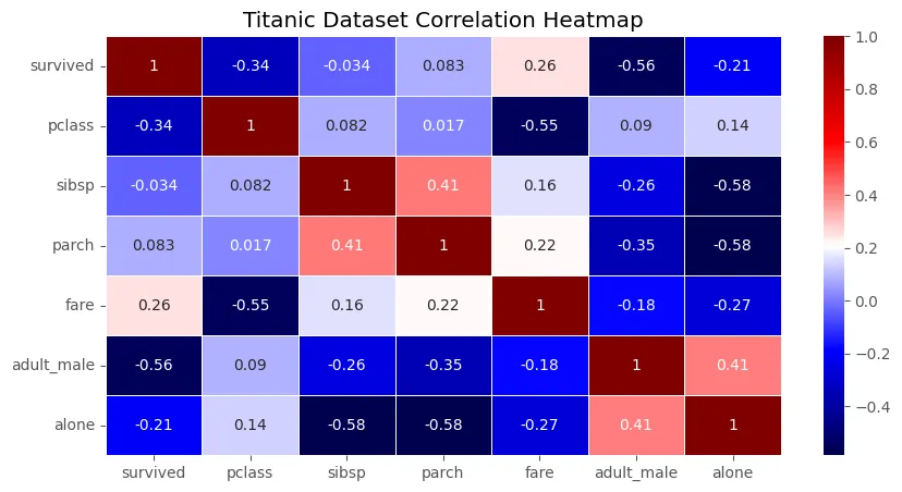
Another powerful tool for exploring relationships is a correlation heatmap, which visualizes the linear relationships between all numerical features.

5. Final Preparation: Separating Features and Target

The final step in preparing our data is to separate the columns we will use to make predictions (the features) from the column we are trying to predict (the target).

• Features (X): All the columns we want to use as input to our model. We will also drop columns that are not useful for prediction, such as PassengerId, Name, and Ticket.
• Target (y): The Survived column, which is the output our model will try to predict.

At this point, our dataset is fully loaded, inspected, cleaned, and prepared. The next logical step in a full project would be to split this data into training and testing sets using Scikit-learn's train_test_split, which you learned about in the previous lesson. However, our goal for this lesson was preparation, and we have achieved it.

Conclusion

Congratulations on completing your first data science project! You have successfully navigated the entire Exploratory Data Analysis workflow, transforming a raw dataset into a clean, well-understood, and model-ready format.

Key Takeaways:

• EDA Workflow: A structured process of loading, inspecting, cleaning, and visualizing data is fundamental to any data science project.
• Data Cleaning: We addressed real-world data imperfections by handling missing values (dropping or imputing) and encoding categorical variables.
• Insight through Visualization: We used countplot and heatmaps to move beyond raw numbers and uncover significant patterns, such as the relationship between sex, class, and survival.
• Preparation for Modeling: The final dataset is separated into a feature matrix X and a target vector y, the standard input format for Scikit-learn models.

This lesson marks the end of our first module. You are now equipped with the essential Python toolkit for any data scientist.

Preview of the Next Module:
Now that we know how to prepare data, we will turn our attention to the models themselves. In the next module, "Probability Models for Data," we will dive into the mathematical foundations of data science, starting with the probability distributions that are used to model real-world phenomena.