L1 vs. L2 Regularization: Impact on Coefficients

Introduction

Welcome back! In our last lesson, we took a deep dive into Ridge Regression. We derived its closed-form solution and saw how its L2 penalty shrinks model coefficients towards zero, providing a powerful mechanism to reduce variance and improve model stability, especially in the presence of multicollinearity.

This lesson builds directly on that foundation by introducing a popular alternative: Lasso (Least Absolute Shrinkage and Selection Operator) Regression. Lasso uses an L1 penalty, and this seemingly minor change in the penalty term—from squared coefficients to absolute values of coefficients—has a profound and fascinatingly different effect.

Our objective is to understand precisely how and why L1 (Lasso) and L2 (Ridge) regularization affect model coefficients differently. By the end of this lesson, you will be able to explain this distinction from three complementary perspectives, satisfying your request for mathematical, geometric, and intuitive insights:

An analytical view, by examining the derivatives of the penalty terms.
A geometric view, by comparing their constraint regions.
A probabilistic view, by interpreting them as Bayesian MAP estimation with different prior beliefs.

1. The Lasso (L1) and Ridge (L2) Cost Functions

Let's start by placing the cost functions side-by-side. Both begin with the Ordinary Least Squares (OLS) Residual Sum of Squares (RSS), but they add a different penalty on the coefficient vector $θ$ .

Ridge (L2) Cost Function:

J_{R i d g e} (θ) = RSS i = 1 \sum m (y_{i} - x_{i}^{T} θ)^{2} + λ L2 Penalty j = 1 \sum n θ_{j}^{2}

Lasso (L1) Cost Function:

J_{L a sso} (θ) = RSS i = 1 \sum m (y_{i} - x_{i}^{T} θ)^{2} + λ L1 Penalty j = 1 \sum n ∣ θ_{j} ∣

The key difference lies in the penalty term:

L2 Penalty (Ridge): The sum of the squared coefficients, also known as the squared L2-norm $∥ θ ∥_{2}^{2}$ .
L1 Penalty (Lasso): The sum of the absolute values of the coefficients, also known as the L1-norm $∥ θ ∥_{1}$ .

This difference completely changes the nature of the solution. To build your intuition, let's start with a visual exploration of how these penalties alter the shape of the cost function.

Ridge vs Lasso Regression, Visualized!!!

This video from StatQuest provides an excellent visualization of how the L1 and L2 penalties modify the original sum-of-squared-residuals curve.

Watch the video from 02:19 to 08:33. Pay close attention to the visual difference between the resulting curves. Notice how the L2 penalty keeps the curve smooth and parabolic, merely shifting the minimum. In contrast, observe how the L1 penalty introduces a sharp 'kink' at zero, which is the key to its unique behavior.

As the video demonstrates, the L1 penalty's "kink" at zero allows the minimum of the cost function to fall precisely at zero for a large enough $λ$ . The L2 penalty, being smooth, only pushes the minimum towards zero. Now, let's explore why this happens.

2. The Analytical View: A Tale of Two Derivatives

The most direct way to understand the different behaviors is to inspect the gradient of the penalty terms. During optimization (e.g., using gradient descent), the update for each coefficient $θ_{j}$ includes a term from the regularization penalty's derivative.

L2 (Ridge) Gradient

The L2 penalty for a single coefficient is $λ θ_{j}^{2}$ . Its derivative with respect to $θ_{j}$ is:

\frac{\partial}{\partial θ _{j}} (λ θ_{j}^{2}) = 2 λ θ_{j}

This derivative is proportional to $θ_{j}$ . This means:

If $θ_{j}$ is large, the "pull" towards zero is strong.
As $θ_{j}$ approaches zero, the "pull" from the penalty term also approaches zero ( $2 λ θ_{j} \to 0$ ).

The regularization's effect diminishes as the coefficient gets smaller. It acts like a spring whose restoring force weakens as it gets closer to its equilibrium point. It pulls coefficients close to zero, but it rarely has the final "push" to make them exactly zero.

L1 (Lasso) Gradient

The L1 penalty is $λ ∣ θ_{j} ∣$ . This function is not differentiable at $θ_{j} = 0$ . However, we can analyze its subgradient, which for $θ_{j} \neq = 0$ is:

\frac{\partial}{\partial θ _{j}} (λ ∣ θ_{j} ∣) = λ \cdot sign (θ_{j}) = {+ λ - λ if θ_{j} > 0 if θ_{j} < 0

Notice the crucial difference: the gradient is constant. It does not depend on the magnitude of $θ_{j}$ .

The "pull" towards zero is always a constant $λ$ , no matter how small $θ_{j}$ becomes (as long as it's not zero).

This constant force will eventually drag the coefficient all the way to zero and hold it there. This property is why Lasso performs feature selection: by setting coefficients to zero, it effectively removes irrelevant features from the model.

L1 vs L2 Regularization: Intuition, Geometry, and Bayesian View

The following article provides a concise textual explanation of this derivative-based intuition.

Read the sections 'L2: Smooth Shrinkage' and 'L1: Constant Push Toward Zero'. This will reinforce the mathematical reason why L2 shrinks smoothly while L1 pushes coefficients all the way to zero.

3. The Geometric View: Circles vs. Diamonds

A powerful and elegant way to visualize the difference is to reframe regularization as a constrained optimization problem.

Ridge Regression is equivalent to minimizing the RSS subject to the constraint $\sum θ_{j}^{2} \leq t$ , which defines a circle (in 2D) or a hypersphere (in higher dimensions).
Lasso Regression is equivalent to minimizing the RSS subject to the constraint $\sum ∣ θ_{j} ∣ \leq t$ , which defines a diamond (in 2D) or a cross-polytope (in higher dimensions).

The optimal solution is the point where the elliptical contours of the RSS function first touch the boundary of the constraint region.

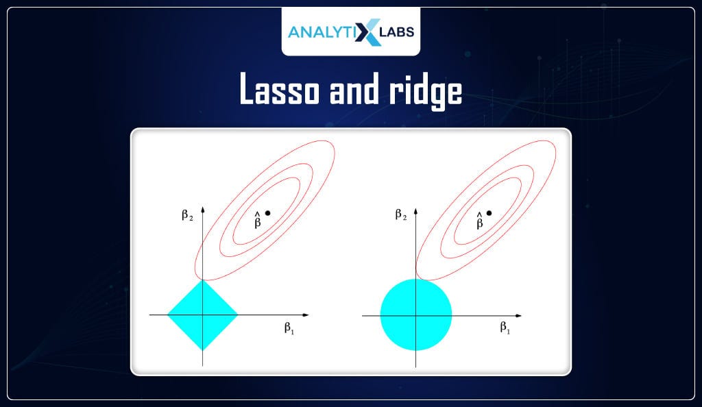
Geometric Interpretation of Lasso and Ridge Regression — A comparison of Lasso (L1) and Ridge (L2) regularization. The solution is the point where the red RSS ellipses first touch the blue constraint region. The circular L2 boundary tends to be touched at points where no coefficient is zero. The sharp corners of the L1 diamond lie on the axes, making it highly probable that the solution will be at a corner, forcing one coefficient to be exactly zero.

As the image shows, the expanding RSS ellipses are much more likely to intersect the L1 diamond at one of its corners. Since these corners lie on the axes (e.g., where $θ_{1} = 0$ ), the solution will be sparse. The smooth, circular boundary of the L2 constraint has no corners, so the intersection typically occurs at a point where both coefficients are non-zero.

This geometric perspective gives a strong intuitive reason for Lasso's sparsity-inducing property.

Sparsity and the L1 Norm

The following video provides an excellent animated explanation of this geometric viewpoint.

Watch the segment from 00:44 to 09:02. The presenter provides a fantastic walkthrough of how minimizing a function subject to different norm constraints leads to different solutions. Focus on the visualization of 'growing' the norm balls until they intersect the solution line.

4. The Probabilistic View: Gaussian vs. Laplace Priors

Finally, we can interpret regularization through a Bayesian lens, which connects it to the fundamental principles of statistical inference you've been studying. Regularization is equivalent to performing Maximum A Posteriori (MAP) estimation, where we assume a prior probability distribution over the model's weights.

The MAP estimate is found by minimizing the negative log-posterior:

θ^_{M A P} = ar g θ min [- lo g P (Data ∣ θ) - lo g P (θ)]

Here, $- lo g P (Data ∣ θ)$ is the negative log-likelihood (which corresponds to the RSS term for Gaussian noise), and $- lo g P (θ)$ is the regularization term derived from our prior belief about the weights.

Ridge (L2): If we assume the weights follow a Gaussian (Normal) prior, $P (θ) \sim N (0, σ^{2})$ , then its negative log-probability is proportional to $θ^{2}$ .
$- lo g P (θ) \propto θ^{2} ⟹ L2 Penalty$
A Gaussian prior assumes that weights are likely to be small and clustered around zero, but it assigns very low probability to any single value, including exactly zero.
Lasso (L1): If we assume the weights follow a Laplace prior, $P (θ) \sim Laplace (0, b)$ , then its negative log-probability is proportional to $∣ θ ∣$ .
$- lo g P (θ) \propto ∣ θ ∣ ⟹ L1 Penalty$
The Laplace distribution is sharply peaked at zero. This represents a much stronger prior belief that many of the coefficients are exactly zero.

[PDF] Understanding L1 and L2 regularization with analytical and probabilistic views

For a rigorous mathematical derivation of these probabilistic connections, the following PDF is an excellent resource.

Read section '2.2 Probabilistic derivation of L1 regularization' and section '3.2 Probabilistic derivation of L2 regularization'. These sections formally show how assuming a Laplace prior for the weights leads to the L1 penalty, and a Gaussian prior leads to the L2 penalty, when performing MAP estimation.

Summary of Differences

This table summarizes the key distinctions between Lasso and Ridge regularization.

Feature	Ridge (L2) Regularization	Lasso (L1) Regularization
Penalty Term	$λ \sum θ_{j}^{2}$ (Sum of squares)	$\lambda \sum
Sparsity	No. Shrinks coefficients towards zero, but they rarely become exactly zero.	Yes. Can shrink coefficients to be exactly zero.
Effect	Primarily reduces model complexity by shrinking coefficients. Useful for multicollinearity.	Performs feature selection by eliminating useless features.
Solution	Has a closed-form solution.	No general closed-form solution. Requires numerical optimization.
Geometry	Constraint region is a circle/sphere.	Constraint region is a diamond/cross-polytope.
Bayesian Prior	Gaussian prior on coefficients.	Laplace prior on coefficients.
Main Use Case	When you have many features with small to medium effects.	When you suspect many features are irrelevant.

A popular hybrid of the two is Elastic Net, which includes both L1 and L2 penalty terms, offering a balance of feature selection and coefficient shrinkage.

Conclusion

You have now explored the critical differences between L1 and L2 regularization from multiple angles. This multi-faceted understanding is key to not only using these techniques effectively but also to appreciating the elegance and interconnectedness of concepts in machine learning.

Key Takeaways:

Ridge (L2) uses a squared penalty ( $θ^{2}$ ) which results in a smooth gradient. This shrinks all coefficients proportionally but rarely sets any to exactly zero. It's excellent for handling multicollinearity when you believe all features contribute.
Lasso (L1) uses an absolute value penalty ( $∣ θ ∣$ ) which has a constant gradient. This provides a consistent push towards zero, resulting in sparsity and performing automatic feature selection.
Geometrically, the smooth, circular L2 constraint encourages shrinkage, while the sharp, cornered L1 diamond promotes solutions where some coefficients are zero.
From a Bayesian perspective, L2 corresponds to a Gaussian prior on the weights, while L1 corresponds to a Laplace prior, which expresses a stronger belief in sparse coefficients.

Preview of the Next Lesson:

Theory is powerful, but seeing it in action solidifies understanding. In the next lesson, we will embark on a hands-on project. You will build and evaluate a regularized linear model using Python's Scikit-learn library. You'll apply both Ridge and Lasso to a real-world dataset, analyze the effect of the regularization parameter $λ$ on the coefficients, and see firsthand how Lasso performs feature selection.

Recommended resources