Linear Regression with NumPy and Gradient Descent

Introduction

Welcome to a new module focused on building predictive models. In the previous module, we explored hypothesis testing, a framework for determining if observed differences in data are statistically significant. We used tools like the t-test and Chi-square test to answer questions like, "Is group A different from group B?"

Now, we shift our focus from identifying differences to modeling relationships. Our goal is to create functions that can predict an outcome based on input features. We'll begin with the most fundamental and widely used model in all of data science: Linear Regression.

Your background in engineering has likely involved fitting lines to experimental data to understand trends. In this lesson, we will formalize that process into a machine learning algorithm. Our objective is to not just use a pre-built library function, but to implement linear regression from scratch using NumPy. This will give you a deep, first-principles understanding of how a model learns from data. We will cover the model's mathematical formulation, define a cost function to measure its error, and implement the gradient descent algorithm to find the optimal model parameters.

1. The Linear Regression Model

The core idea of linear regression is to model the relationship between an input variable (or variables), called features, and a continuous output variable, called the target, by fitting a linear equation to the observed data.

1.1 The Hypothesis Function

In machine learning, this linear equation is called the hypothesis function, denoted as $h_{θ} (x)$ . For a single input feature $x$ , the hypothesis is:

h_{θ} (x) = θ_{0} + θ_{1} x

Here:

$x$ is the input feature (e.g., size of a house).
$y$ is the target variable we want to predict (e.g., price of the house).
$θ_{0}$ is the bias or intercept term (the value of $y$ when $x = 0$ ).
$θ_{1}$ is the weight for the feature $x$ (the slope of the line).

The vector $θ = [θ_{0}, θ_{1}]$ contains the parameters of our model. The goal of "learning" is to find the values of $θ$ that make the line $h_{θ} (x)$ best fit the training data.

1.2 The Cost Function: Measuring Error

To find the "best" parameters, we first need a way to quantify how well a given line fits the data. We do this with a cost function (or loss function), which measures the difference between the model's predictions and the actual target values.

For linear regression, the standard cost function is the Mean Squared Error (MSE), denoted as $J (θ)$ . It calculates the average of the squared differences between the predicted values $h_{θ} (x^{(i)})$ and the actual values $y^{(i)}$ for all $m$ training examples.

J (θ) = \frac{1}{2 m} i = 1 \sum m (h_{θ} (x^{(i)}) - y^{(i)})^{2}

The factor of $\frac{1}{2}$ is included for mathematical convenience, as it simplifies the derivative we will take later. Our goal is to find the $θ$ that minimizes this cost function $J (θ)$ .

To get a formal introduction to these concepts, let's watch the classic lecture from Andrew Ng's Machine Learning course at Stanford.

Stanford CS229: Machine Learning - Linear Regression and Gradient Descent | Lecture 2 (Autumn 2018)

This video provides a rigorous introduction to the linear regression model. It defines the hypothesis function, the parameters, and the Mean Squared Error cost function.

Watch the video from 01:33 to 17:52. Pay close attention to: The notation used for the training set, parameters ( heta), and hypothesis (h). The generalization from a single feature to multiple features. The mathematical formulation of the cost function, J(\theta), and why we aim to minimize it.

2. Optimization with Gradient Descent

Now that we have a cost function $J (θ)$ that measures our model's error, how do we find the values of $θ$ that minimize it? The answer is an optimization algorithm called Gradient Descent.

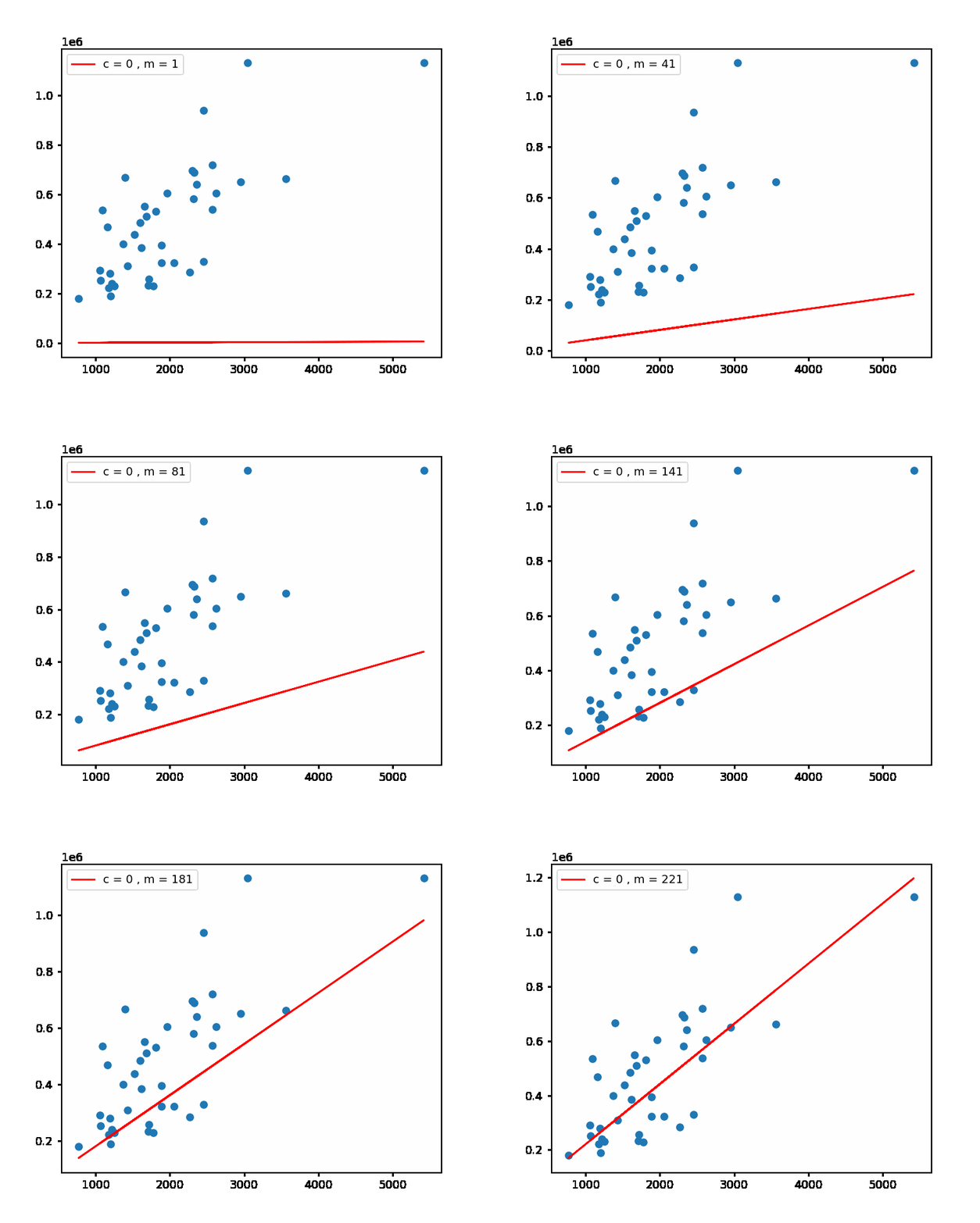
Imagine the cost function $J (θ)$ as a bowl-shaped surface. The horizontal axes represent the parameters ( $θ_{0}, θ_{1}$ ), and the vertical axis represents the cost $J$ . Our goal is to find the point at the very bottom of this bowl.

Gradient descent does this by starting at some random point on the surface and iteratively taking small steps in the direction of the steepest descent, i.e., downhill.

Linear Regression with Gradient Descent Animation — This animation shows how gradient descent works. The red line represents our model's hypothesis. It starts with a random guess for the parameters (slope and intercept) and iteratively adjusts them to better fit the data points, minimizing the error at each step.

2.1 The Gradient Descent Algorithm

The algorithm works as follows: we repeatedly update each parameter $θ_{j}$ by subtracting the partial derivative of the cost function with respect to that parameter, scaled by a learning rate $α$ .

The update rule for each parameter $θ_{j}$ is:

θ_{j} := θ_{j} - α \frac{\partial}{\partial θ _{j}} J (θ)

The := symbol denotes assignment.
$α$ is the learning rate, a hyperparameter that controls the size of each step.
$\frac{\partial}{\partial θ _{j}} J (θ)$ is the partial derivative (the gradient), which tells us the direction of steepest ascent. We move in the opposite direction to go downhill.

Gradient Descent Algorithm for Linear Regression — This image summarizes the gradient descent update rules for parameters $\theta_0$ and $\theta_1$. Notice the instruction for 'simultaneous update,' which is crucial for the algorithm's correctness.

2.2 Deriving the Gradient

To implement this, we need to calculate the partial derivatives of our cost function $J (θ)$ . Let's derive them.

Our cost function is:

J (θ_{0}, θ_{1}) = \frac{1}{2 m} i = 1 \sum m (θ_{0} + θ_{1} x^{(i)} - y^{(i)})^{2}

Using the chain rule of calculus, we find the partial derivatives:

For $θ_{0}$ :

\frac{\partial}{\partial θ _{0}} J (θ_{0}, θ_{1}) = \frac{1}{2 m} i = 1 \sum m 2 (θ_{0} + θ_{1} x^{(i)} - y^{(i)}) \cdot 1 = \frac{1}{m} i = 1 \sum m (h_{θ} (x^{(i)}) - y^{(i)})

For $θ_{1}$ :

\frac{\partial}{\partial θ _{1}} J (θ_{0}, θ_{1}) = \frac{1}{2 m} i = 1 \sum m 2 (θ_{0} + θ_{1} x^{(i)} - y^{(i)}) \cdot x^{(i)} = \frac{1}{m} i = 1 \sum m (h_{θ} (x^{(i)}) - y^{(i)}) x^{(i)}

Now, we can plug these back into our update rules:

Repeat until convergence {

θ_{0} := θ_{0} - α \frac{1}{m} i = 1 \sum m (h_{θ} (x^{(i)}) - y^{(i)})

θ_{1} := θ_{1} - α \frac{1}{m} i = 1 \sum m (h_{θ} (x^{(i)}) - y^{(i)}) x^{(i)}

}

This form of gradient descent, which uses all $m$ training examples in each update step, is known as Batch Gradient Descent.

The following video provides a detailed walk-through of the gradient descent intuition and the derivation of the update rule.

Stanford CS229: Machine Learning - Linear Regression and Gradient Descent | Lecture 2 (Autumn 2018)

This next segment of the Stanford lecture explains the intuition behind gradient descent, derives the update rule mathematically, and discusses practical considerations like choosing the learning rate and the difference between batch and stochastic gradient descent.

Watch from 17:52 to 53:04. This is a crucial section. Focus on: Intuition (17:52 - 22:49): The visualization of minimizing the cost function by taking steps downhill. Mathematical Derivation (22:49 - 32:56): Follow the derivation of the partial derivatives for the gradient descent update rule. This will match the derivation we just did. Convergence and Learning Rate (33:34 - 39:08): Understand why linear regression's cost function is convex and how the choice of learning rate \alpha affects convergence. Batch vs. Stochastic Gradient Descent (40:54 - 53:04): Grasp the key difference between using the entire dataset (batch) versus one example at a time (stochastic) for updates, and the trade-offs involved.

3. Project: Implementing Linear Regression from Scratch

Now it's time to translate this theory and math into working code. We will implement Batch Gradient Descent for linear regression using only NumPy.

This video tutorial provides an excellent, step-by-step guide to building the model from scratch. We'll follow its structure.

Multiple Linear Regression with Gradient Descent from Scratch

This tutorial by Kody Simpson is a practical guide to implementing linear regression and gradient descent. It starts with the basics and builds a complete, working model in Python.

For this section, please set up a Python notebook and follow along with the video from 02:23 to 23:46. Then, jump to the implementation part from 33:47 to 46:09. Understand the Notation (02:23 - 07:45): See how the standard line equation y = mx + b is transformed into the machine learning hypothesis notation y_hat = theta_0 + theta_1 * x_1 and then to a vectorized form. Calculus Refresher (13:28 - 17:52): A quick, intuitive review of derivatives and partial derivatives, which are the engine of gradient descent. Gradient Descent Logic (17:52 - 23:46): Understand the iterative steps of the algorithm before coding it: initialize parameters, calculate the gradient, and update the parameters. Code Implementation (33:47 - 46:09): This is the core task. Follow the video to write the gradient_descent function. Pay special attention to how the mathematical formulas for the partial derivatives are translated into NumPy code. Replicate this in your own notebook.

Let's break down the implementation you just created.

Your `gradient_descent` function should contain the following logic inside a loop:

Get Data Ready:
- You have your feature matrix X (with a column of ones for $θ_{0}$ ) and your target vector y.
- Initialize your parameters $θ$ with random values or zeros.
- Define your hyperparameters: learning rate alpha and number of iterations epochs.
Calculate Predictions: Inside the loop, for the current $θ$ , calculate the predictions for all training examples. In vectorized form, this is a simple matrix-vector multiplication:
```
predictions = X.dot(theta)
```
Calculate Gradients: Compute the partial derivatives for each parameter. The formulas we derived can be vectorized for efficiency. For a model with n features (and thus n+1 parameters), the gradient vector can be computed in one go:
$gradient = \frac{2}{m} \cdot X^{T} \cdot (X θ - y)$
In NumPy, this translates to:
```
errors = predictions - y
gradient = (2/m) * X.T.dot(errors)
```
(Note: The video may implement this slightly differently by calculating gradients for $θ_{0}$ and $θ_{1}$ separately, which is also correct for a simple case. The vectorized form is more general and efficient.)
Update Parameters: Update the $θ$ vector by taking a step in the opposite direction of the gradient:
```
theta = theta - alpha * gradient
```

By running this loop for a set number of iterations, your $θ$ parameters will gradually converge to values that minimize the cost function.

4. Visualizing the Learning Process

A great way to verify that your algorithm is working is to track the cost at each iteration. If gradient descent is working correctly, the cost should decrease over time and eventually plateau.

Task:
Modify your gradient_descent function to calculate and store the MSE cost $J (θ)$ at the end of each iteration. After the loop finishes, plot the cost versus the iteration number. You should see a curve that starts high and rapidly drops, then flattens out.

The Kody Simpson video demonstrates exactly how to do this.

Multiple Linear Regression with Gradient Descent from Scratch

This final clip shows how to track and plot the cost (MSE) over epochs to visualize the learning curve of your model.

Watch from 46:09 to 52:43. Implement the changes to your function to store the error at each epoch and then plot the error curve. Experiment with different learning rates (\alpha) and numbers of epochs to see how they affect the learning curve, just as shown in the video.

Conclusion

Excellent work! You have successfully built a fundamental machine learning algorithm from the ground up. You have not only implemented linear regression but also gained a deep understanding of the core components that drive many other machine learning models.

Key Takeaways:

Linear Regression Model: A simple yet powerful model represented by the hypothesis function $h_{θ} (x) = X θ$ .
Cost Function: The Mean Squared Error (MSE), $J (θ)$ , quantifies the model's error and provides a target for optimization.
Gradient Descent: An iterative optimization algorithm that minimizes the cost function by repeatedly updating parameters in the direction opposite to the gradient.
Implementation from Scratch: You translated the mathematical formulas for the model, cost, and gradient descent update rule into working Python code using NumPy, solidifying your understanding of each component.
Hyperparameters: You experimented with the learning rate ( $α$ ) and number of iterations, observing their critical impact on the model's training process.

This foundational knowledge of modeling, cost functions, and optimization is not limited to linear regression; it is the blueprint for many advanced algorithms, including neural networks.

Preview of the Next Lesson:

Now that we can build a model, a natural question arises: how do we know if our model is good? A model that fits the training data perfectly might fail spectacularly on new, unseen data. In the next lesson, we will explore this critical concept by mathematically decomposing a model's generalization error into its Bias, Variance, and Irreducible Noise components. This "Bias-Variance Tradeoff" is a central principle in machine learning that will help you understand the dangers of model underfitting and overfitting.

Recommended resources