Hello! Welcome back to our final lesson on clustering.
In our last two lessons, we delved into the mechanics of two fundamental clustering algorithms. We started with K-means, understanding its geometric interpretation as a partitioning of space into Voronoi cells, leading to "hard" cluster assignments. Then, we tackled the mathematically rich Gaussian Mixture Model (GMM), deriving the Expectation-Maximization (EM) algorithm that allows for "soft," probabilistic assignments.
Now, we will synthesize this knowledge. Our goal today is to compare and contrast the use cases for K-means versus GMMs. This lesson will move from the "how" to the "when and why," equipping you to choose the right tool for a given clustering problem.
1. The Limitations of a Center-Based Approach
As we saw, K-means defines clusters solely by their centroids. It assigns each point to the single, closest centroid. This is fast and intuitive, but it carries two major, implicit assumptions:
- Clusters are spherical (or hyperspherical in more dimensions).
- All clusters have a similar size/variance.
What happens when these assumptions are violated? The model can fail to capture the true underlying structure of the data.
Let's start by reading a resource that illustrates these weaknesses.
In Depth: Gaussian Mixture Models
The 'Python Data Science Handbook' by Jake VanderPlas provides an excellent, code-driven explanation of K-means' limitations. This section will demonstrate how its reliance on circular cluster models can lead to poor results on non-circular data.
Read the section 'Motivating GMM: Weaknesses of k-Means'. Pay close attention to the two key weaknesses identified: the lack of probabilistic assignment and the inflexibility in cluster shape. Examine the code and the resulting plots, especially the one with the stretched data, to see a concrete example of K-means failing.
The resource highlights two main issues:
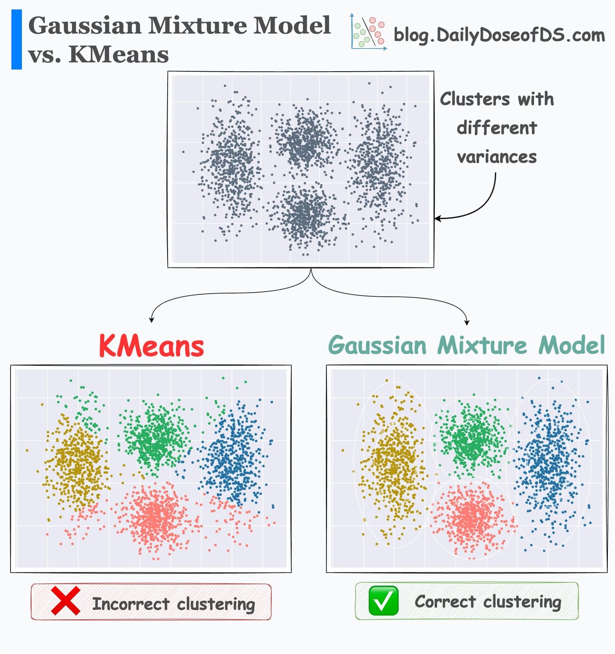
- Lack of Flexibility in Cluster Shape: K-means forces data into circular "molds." If your data forms elongated or elliptical groups, K-means will likely misclassify points where these underlying shapes overlap.
- Lack of Probabilistic Assignment: K-means provides a hard assignment. For a point lying between two clusters, it gives no measure of uncertainty about the assignment. A probabilistic assignment would be more informative.
The following image illustrates this fundamental difference between "hard" and "soft" clustering.

2. GMM: A More Flexible, Probabilistic Approach
Gaussian Mixture Models directly address the shortcomings of K-means. A GMM assumes that the data is generated from a mixture of Gaussian distributions, each with its own mean, covariance, and weight.
This has two powerful consequences:
- Flexible Cluster Shapes: By using a full covariance matrix for each component, GMMs can model clusters that are elliptical and oriented in any direction.
- Probabilistic Assignments: As we derived in the last lesson, the output of the E-step is a set of "responsibilities"—the probability of each point belonging to each cluster. This provides a natural way to express uncertainty.
Let's see how GMM handles the exact situations where K-means struggled.
In Depth: Gaussian Mixture Models
Now, let's continue in the same 'Python Data Science Handbook' article to see how GMMs overcome the limitations we just saw.
Read the section 'Generalizing E–M: Gaussian Mixture Models'. Notice how GMMs successfully model both the simple and the stretched datasets. Pay particular attention to the predict_proba method and the visualization that uses point sizes to represent uncertainty.
The image below provides another stark visual comparison.
3. Core Differences: A Head-to-Head Comparison
Let's formalize our comparison. The following video gives a great conceptual overview of the differences.
What are Gaussian Mixture Models? | Soft clustering | Unsupervised Machine Learning | Data Science
This video provides a concise summary of why GMMs are needed and how they differ from K-means. It reinforces the ideas of soft clustering and the probabilistic model.
Watch the first minute (0:00-1:06) to see the problem setup, and then the summary from 7:34 to 9:39, which directly compares the two methods.
Now, let's dive deeper into the relationship between the algorithms.
Clustering (4): Gaussian Mixture Models and EM
This video from Alexander Ihler frames GMM as a direct extension of K-means and discusses their algorithmic similarities and differences, which will resonate with your interest in the underlying mechanics.
Please watch the following two segments: (0:01 - 2:11): This introduces GMMs by highlighting K-means' limitations with non-circular and overlapping clusters, and explicitly states that K-means can be viewed as a special case of GMM. (5:10 - 8:40): This explains the E and M steps of the EM algorithm for GMMs. Compare this mentally to the two steps of K-means (assign points to clusters, update centroids). Notice the parallel: the E-step is a soft 'assignment', and the M-step is an 'update' of the cluster parameters (mean, covariance, weight).
Based on these resources and our previous lessons, we can build a comprehensive comparison table.
| Feature | K-Means Clustering | Gaussian Mixture Model (GMM) |
|---|---|---|
| Cluster Shape | Assumes spherical, equal-sized clusters. | Can model elliptical clusters of varying sizes and orientations. |
| Assignment | Hard Clustering: Each point belongs to a single cluster. | Soft Clustering: Each point has a probability of belonging to each cluster. |
| Underlying Model | Non-parametric, distance-based algorithm. It finds partitions. | Parametric, generative model. It learns a probability distribution for the data. |
| Output | Cluster labels for each data point. | Cluster probabilities, plus parameters () that describe the data distribution. |
| Complexity | Computationally faster, especially with many dimensions. Scales as . | More computationally expensive due to probability calculations and covariance matrices. Scales as . |
| Key Hyperparameter | Number of clusters, . | Number of components, , and covariance_type. |
(Where is number of samples, is number of clusters, is number of dimensions, and is number of iterations.)
4. Practical Guidelines: When to Use Which?
This comparison leads to clear practical advice.
Choose K-means when:
- Speed is critical: It's significantly faster, making it a great first choice or baseline.
- You have a very large number of features (high D): The term in GMM's complexity can make it unfeasible.
- You have reason to believe clusters are roughly spherical and well-separated.
- Simplicity is valued: The algorithm is easier to understand and implement from scratch.
Choose GMM when:
- Clusters are not spherical: Your data appears elongated or rotated. You can control the flexibility with the
covariance_typehyperparameter ('spherical', 'diag', 'full'), as mentioned in the Python Data Science Handbook reading. - Clusters overlap or have different densities/sizes: GMM's probabilistic nature handles this ambiguity gracefully.
- You need probabilistic assignments: You want to know the uncertainty of a point's classification.
- You want a generative model: Because GMM learns a probability distribution, you can use it to generate new data points that resemble your original dataset. This is a powerful capability that K-means lacks. The
make_moonsexample in the Python Data Science Handbook (resource_id: [LINK](https://jakevdp.github.io/PythonDataScienceHandbook/05.12-gaussian-mixtures.html), section 'GMM as Density Estimation') is a fantastic illustration of this.
5. The Deeper Connection: K-means as a Special Case of GMM
For a final point that touches on your interest in mathematical proofs and connections, it's illuminating to realize that K-means is a special, constrained version of a GMM using the EM algorithm.
Imagine a GMM where:
- The covariance matrix for every component is a spherical identity matrix scaled by the same variance : . This forces all clusters to be spherical and of equal size.
- You let the variance .
As the variance approaches zero, the Gaussian "bells" become infinitely sharp peaks. The responsibility for a data point will become 1 for the nearest cluster and 0 for all others. This hard assignment is exactly the E-step of K-means. The M-step of this GMM, which updates the means, simplifies to just calculating the average of the points assigned to that cluster—exactly the M-step of K-means.
Conclusion
Today we built a practical framework for deciding between K-means and GMM. While both are iterative clustering algorithms, their underlying assumptions lead to different strengths and weaknesses.
Key Takeaways:
- K-means is a fast, simple algorithm ideal for spherical, well-separated clusters, performing hard assignments.
- GMM is a flexible, probabilistic model that can handle elliptical, overlapping clusters of varying sizes, performing soft assignments.
- The core trade-off is speed and simplicity (K-means) versus flexibility and richness of output (GMM).
- GMM is a generative model, meaning it learns the underlying data distribution and can be used to generate new samples. K-means is purely a partitioning algorithm.
Preview of the Next Lesson
We have concluded our module on clustering, where we focused on finding group structures within data. We now pivot to a new topic: dimensionality reduction. In the next lesson, we will begin Module 11 by exploring Principal Component Analysis (PCA). You will see how we can transform high-dimensional data into a lower-dimensional representation while preserving as much information as possible, a technique with deep connections to linear algebra and variance maximization.