Sequential Bayesian Estimation for Coin Bias

1. The Analytical Framework: Beta-Binomial Model

Before we start coding, we need to set up the mathematical model for our coin flip problem. This is analogous to how in engineering, you'd first establish the governing equations of a physical system before simulating it. Our system consists of a coin with an unknown bias $\theta$ (the probability of getting heads), which we want to estimate.

Likelihood: The Data-Generating Process

Each coin flip is an independent event. The outcome of a single flip, which can be either heads (1) or tails (0), is modeled by a Bernoulli distribution:
$p(\text{data}=k|\theta )={\theta }^k(1-\theta {)}^{1-k},k\in \{0,1\}$
When we consider $N$ flips and are interested in the total number of heads, $z$, the likelihood of the data is given by the Binomial distribution.

Prior: Quantifying Our Initial Belief

We need to express our initial belief about the coin's bias, $\theta$. Since $\theta$ must lie between 0 and 1, the Beta distribution is an excellent choice for our prior. It's defined on the interval $[0,1]$ and is highly flexible, controlled by two positive shape parameters, $\alpha$ and $\beta$.
$p(\theta )=\text{Beta}(\theta |\alpha ,\beta )\propto {\theta }^{\alpha -1}(1-\theta {)}^{\beta -1}$
The parameters $\alpha$ and $\beta$ can be thought of as "pseudo-counts" of heads and tails from imagined prior experiments. A prior of $\text{Beta}(1,1)$ is a uniform distribution, representing complete uncertainty. A prior of $\text{Beta}(10,10)$ expresses a belief that the coin is fair, with some confidence.

Posterior: Combining Belief and Evidence

The magic happens when we combine our Beta prior with our Binomial/Bernoulli likelihood. Because the Beta distribution is the conjugate prior for the Binomial/Bernoulli likelihood, the resulting posterior distribution is also a Beta distribution. This conjugacy makes the math remarkably clean.

To see how this works, let's watch a short video that provides the proof.

As the video demonstrated, if we start with a prior $\text{Beta}({\alpha }_{\text{prior}},{\beta }_{\text{prior}})$ and observe data consisting of $z$ heads and $N-z$ tails, our posterior belief is updated to:
$p(\theta |\text{data})=\text{Beta}(\theta |{\alpha }_{\text{prior}}+z,{\beta }_{\text{prior}}+N-z)$
This simple update rule—just adding the observed heads and tails to our prior's parameters—is the core of our Bayesian estimator.

2. The Sequential Update

Our project requires us to update beliefs sequentially, one flip at a time. The Bayesian framework handles this elegantly: the posterior from one step becomes the prior for the next.

Formally, for two conditionally independent observations $x_1$ and $x_2$, the posterior after observing both is:
$p(\theta |x_1,x_2)\propto p(x_2|\theta )\cdot p(\theta |x_1)$
Notice that the term $p(\theta |x_1)$ is the posterior after the first observation, and it acts as the prior for the second observation $x_2$. This is precisely what we will implement.

If our current belief is $\text{Beta}(\alpha ,\beta )$ and the next flip is Heads ($z=1,N-z=0$), our new belief becomes:
$\text{Beta}(\alpha +1,\beta )$
If the next flip is Tails ($z=0,N-z=1$), our new belief becomes:
$\text{Beta}(\alpha ,\beta +1)$

Let's read a short, formal confirmation of this process.

3. Project: Implementing the Sequential Bayesian Estimator

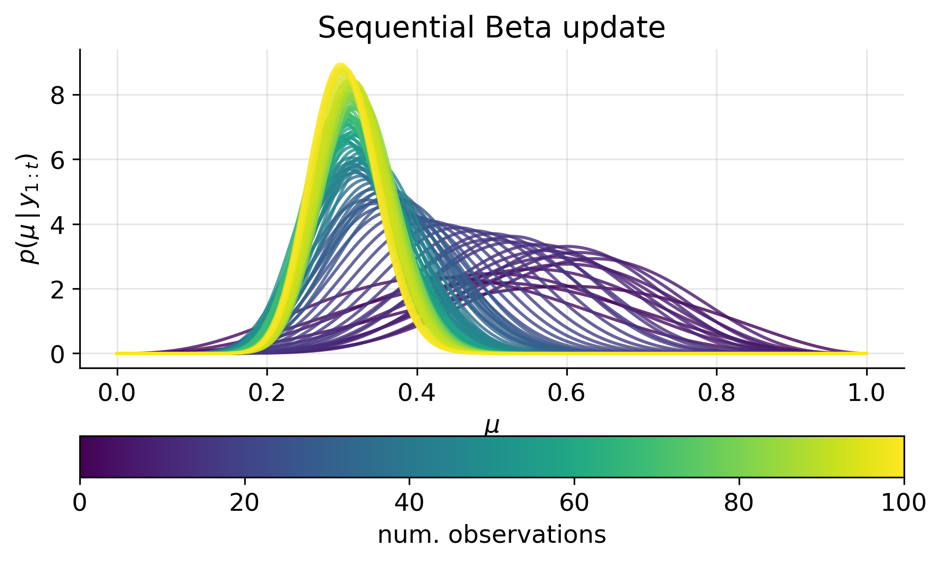
Now it's time to build the estimator. Your task is to write a Python script that simulates a series of coin flips and, after each flip, updates and plots the posterior distribution for the coin's bias $\theta$.

Your final output should resemble this image, which clearly shows the belief distribution narrowing as more data is collected:

Step-by-Step Implementation Guide

Follow these steps to complete the project. I've provided skeleton code for you to fill in.

Step 1: Setup
Import the necessary libraries.

import numpy as np
from scipy.stats import beta
import matplotlib.pyplot as plt
import seaborn as sns




# Set plotting style
sns.set(style='whitegrid')

Step 2: Define Ground Truth and Priors
First, we'll define the true bias of our simulated coin. In a real-world scenario, this would be unknown. We'll also set the parameters for our initial prior belief. A uniform prior, Beta(1, 1), is a good choice to represent initial ignorance.

# True (unknown) probability of heads
theta_true = 0.6




# Generate a sequence of 100 coin flips
np.random.seed(42) # for reproducibility
flips = np.random.binomial(1, theta_true, size=100)




# Prior parameters (alpha and beta)
# A Beta(1, 1) distribution is a uniform distribution on [0, 1]
alpha_prior = 1
beta_prior = 1




# A list of points in time when we want to plot our distribution
plot_points = [0, 1, 2, 5, 10, 20, 50, 100]

Step 3: The Sequential Update Loop
Now, you will loop through the simulated flips. In each iteration, you'll update the alpha and beta parameters and, at specified intervals, plot the resulting posterior distribution.

Your task is to complete the code below.

# --- Your Code Goes Here ---




# Initialize current alpha and beta with prior values
alpha_current = alpha_prior
beta_current = beta_prior




# Create a figure to plot on
plt.figure(figsize=(12, 8))




# Define the x-axis for our plots (the range of possible theta values)
x = np.linspace(0, 1, 1000)




# Loop through the number of flips
for i in range(len(flips) + 1):
    



    # Check if the current flip number is one of our designated plot points
    if i in plot_points:



        # 1. Calculate the PDF of the current Beta distribution
        #    Use the `beta.pdf()` function from scipy.stats.
        #    It takes x, alpha_current, and beta_current as arguments.
        y = beta.pdf(x, alpha_current, beta_current)
        



        # 2. Plot the PDF
        #    Use plt.plot() to plot x against y.
        #    Create a label for the legend, e.g., f'N = {i}, Heads = {alpha_current-alpha_prior}'.
        plt.plot(x, y, label=f'N = {i}, Heads = {int(alpha_current - alpha_prior)}')




    # 3. Update alpha_current and beta_current based on the next flip.
    #    Make sure not to go out of bounds of the `flips` array.
    if i < len(flips):
        if flips[i] == 1: # It was a head
            alpha_current += 1
        else: # It was a tail
            beta_current += 1
            



# Add a vertical line for the true value of theta
plt.axvline(x=theta_true, color='red', linestyle='--', label=f'True θ = {theta_true}')




# Finalize the plot
plt.title('Sequential Bayesian Update of a Coin\'s Bias', fontsize=16)
plt.xlabel('θ (Probability of Heads)', fontsize=12)
plt.ylabel('Probability Density', fontsize=12)
plt.legend()
plt.show()




# After the loop, calculate the final posterior mean
posterior_mean = alpha_current / (alpha_current + beta_current)
print(f"\nAfter 100 flips:")
print(f"True bias: {theta_true}")
print(f"Posterior distribution: Beta(α={alpha_current}, β={beta_current})")
print(f"Posterior Mean (MMSE Estimate): {posterior_mean:.4f}")

Analysis of Results

Once your code is running, observe the output. You should see a series of curves. The first one (N=0) is your flat prior. As more flips are observed, the distribution becomes taller and narrower, homing in on the true value of $\theta =0.6$. This is Bayesian learning in action! Your final posterior mean should be very close to 0.6. This mean is the MMSE estimate of $\theta$, which minimizes the expected squared error.

Conclusion

Congratulations! You have successfully built a Bayesian estimator from the ground up. This project demonstrates the power and elegance of the Bayesian approach to learning from data.

Key Takeaways:

• Sequential Learning: Bayesian inference provides a natural mechanism for updating beliefs incrementally. The posterior after one observation serves as the prior for the next.
• Conjugate Priors: Using a conjugate prior (like Beta for a Binomial likelihood) simplifies the math of Bayesian updating, often leading to simple analytical rules (like adding counts).
• Uncertainty Quantification: The posterior distribution doesn't just give a point estimate (like the mean); its width quantifies our uncertainty. As we gather more data, our uncertainty decreases, and the posterior distribution narrows.
• From Ignorance to Knowledge: You visually witnessed the model's "state of belief" evolving from a uniform "I don't know" to a sharply peaked distribution centered near the true value.

Preview of the Next Lesson:

In this module, we have focused on estimation—finding the value of an unknown parameter. We now transition to the next major topic in the DS 215 syllabus: Statistical Hypothesis Testing. In the next lesson, you will learn to formulate null and alternative hypotheses for a given research question. This marks a shift from asking "What is the value of $\theta$?" to asking "Is $\theta$ equal to 0.5?" We will explore the frequentist framework for making such decisions and understanding the associated risks of being wrong.