Vectorized Numerical Computations with Array Comprehensions and Broadcasting

Arrays in Memory: A Foundation for Performance

Before we manipulate arrays, it's crucial to understand how they are stored in memory. The way data is laid out directly impacts how quickly it can be accessed, especially in nested loops which are common in scientific code. Unlike Python's NumPy, which uses row-major ordering, Julia, along with Fortran and MATLAB, uses column-major ordering.

In a 2D array, this means that elements in the same column are contiguous in memory.

This image illustrates the memory access pattern for row-major order, where elements of a row are contiguous, and column-major order, where elements of a column are contiguous. In Julia, the most efficient way to traverse a multi-dimensional array is to have the first index change the fastest in your loops.

To understand why this matters for performance, it's helpful to consider the computer's memory hierarchy—from fast, small caches close to the processor to slower, larger main memory (RAM). Accessing memory sequentially is much faster because the processor can predictively load chunks of data into its cache. Violating this natural memory order leads to "cache misses," which can significantly slow down your code.

The following video provides an excellent explanation of this memory model and demonstrates the performance impact of looping over an array in the correct (column-major) versus incorrect (row-major) order.

The key takeaway is this: When iterating over multi-dimensional arrays in Julia, structure your loops so that the first index changes most rapidly.

For a 2D array A, this means the loop order should be:

for j in 1:size(A, 2)      # Outer loop over columns
    for i in 1:size(A, 1)  # Inner loop over rows
        # do something with A[i, j]
    end
end

This ensures you are "walking" through memory the way the data is laid out, maximizing cache efficiency.

Vectorization and Loop Fusion with Broadcasting

While writing explicit loops is sometimes necessary, Julia provides a more powerful and expressive way to perform element-wise operations: broadcasting. This allows you to apply functions to every element of an array, or combine arrays of different (but compatible) sizes in an element-wise fashion, without writing an explicit loop.

The mechanism for this is the dot (.) syntax. For any function f and operator +, f.(A) applies f to each element of A, and A .+ B performs element-wise addition.

Broadcasting isn't just syntactic sugar for a loop; it's a signal to Julia's compiler to perform an optimization called loop fusion. When you chain multiple broadcasted operations, like Y = a .* X .+ b, Julia doesn't create a temporary array for a .* X and then add b. Instead, it compiles a single, optimized loop that computes a*x[i] + b for each element and writes the result directly to Y. This avoids unnecessary memory allocations and passes over the data, resulting in significantly faster code.

The following image illustrates the rules Julia uses to "stretch" or "broadcast" smaller arrays to match the shape of larger arrays during these operations.

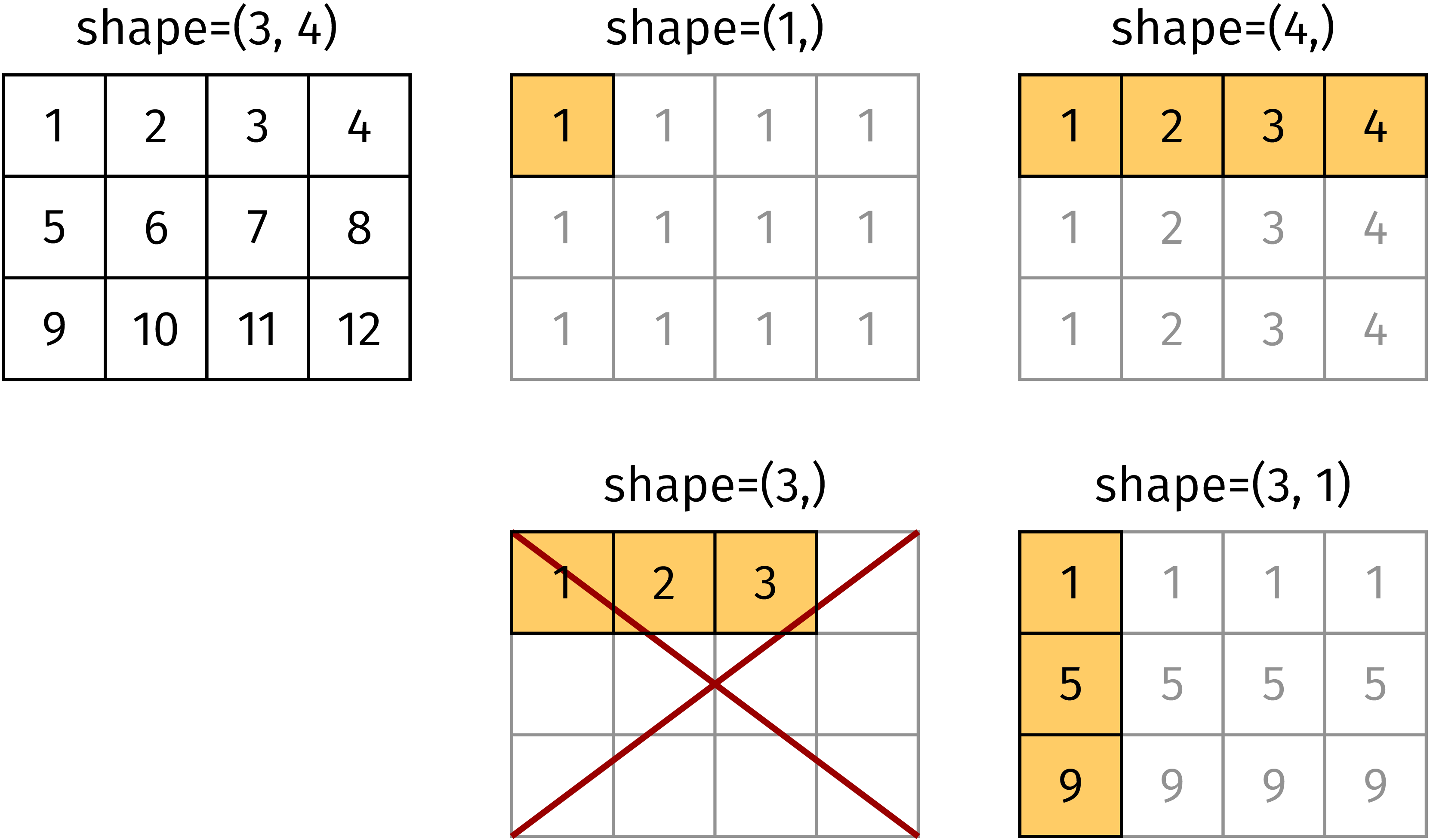
This diagram shows several examples of broadcasting a smaller array onto a 3x4 matrix. A scalar (shape (1,)), a row vector (shape (4,)), and a column vector (shape (3,1)) can all be validly broadcast. However, an array with an incompatible dimension, like the shape (3,) vector, cannot be broadcast against a 2D matrix.

Let's watch another segment of the "Optimizing Serial Code in Julia 1" video to see a detailed breakdown of how loop fusion works and why it's so important for performance.

In-place Operations

A crucial aspect of optimization, especially inside performance-critical loops, is avoiding memory allocation altogether. Broadcasting can be combined with the assignment operator to perform an in-place or mutating operation.

The syntax Y .= a .* X .+ b tells Julia to perform the fused broadcast operation and store the results directly into the pre-existing array Y, overwriting its contents. This completely avoids allocating a new array for the result. By convention, functions that modify their inputs have names ending in an exclamation mark (!), like LinearAlgebra.axpy!. The .= syntax is the broadcasted equivalent for this pattern.

To see the dramatic effect of these different strategies, let's look at a practical example: the AXPY operation (a*x + y).

Concise Array Construction with Comprehensions

The second major tool for vectorized computation is the array comprehension. This provides a concise and readable syntax for constructing an array, and will likely feel familiar from your experience with Python. Comprehensions are ideal for initializing arrays based on their indices, such as setting up a coordinate grid or a potential energy function.

For example, to create a 2D grid representing a potential $V(i,j)=\sin (i)+\cos (j)$, you can simply write:

V = [sin(i) + cos(j) for i in 1:10, j in 1:10]

Julia also has generators, which use the same syntax but with parentheses (). These lazily produce values on demand without allocating the full array, which is useful when you want to iterate over values without storing them, for instance sum(i^2 for i in 1:1000).

This example of building a lattice is a direct first step towards many problems you'll encounter in condensed matter physics.

Summary

In this lesson, we have laid the groundwork for writing high-performance numerical code in Julia. You are now equipped with the essential concepts and tools for efficient array manipulation.

Key Takeaways:

• Column-Major Order: Julia stores arrays with elements in the same column contiguously. Always loop with the first index changing fastest to maximize cache performance.
• Broadcasting with .: Use the dot syntax to apply functions and operators element-wise. This is more than just convenience; it enables loop fusion.
• Loop Fusion: Julia's JIT compiler combines chains of broadcasted operations into a single, efficient loop, avoiding temporary arrays and memory allocations.
• In-place Mutation with .=: For maximum performance, use .= to write the results of a broadcasted operation into a pre-allocated array, eliminating allocations entirely.
• Array Comprehensions: Use the [...] syntax for a concise and readable way to construct arrays, especially for initializing grids and potentials based on their indices.

In our next lesson, we will continue building our toolkit by exploring the LinearAlgebra.jl package. We will move from element-wise operations to the core routines of numerical linear algebra, such as matrix factorizations (LU, QR, SVD), which are fundamental for solving the systems of equations that appear constantly in theoretical physics.