Saving and Loading Scientific Data

Why Not Just Text Files?

In many of your research projects, you've likely dealt with data. For simple datasets, a CSV (Comma-Separated Values) or other delimited text file works well. However, when dealing with the output of large-scale numerical simulations, these formats quickly show their limitations. They are inefficient for storing large arrays of numbers, and more importantly, they cannot natively represent the rich data structures used in Julia. How would you save a custom struct for a tight-binding model, a set of parameters, and the resulting complex-valued eigenvector matrix in a single, organized file?

This is where binary serialization formats become essential. They store data in a way that is much closer to its in-memory representation, making them compact, fast to read and write, and capable of preserving complex, nested data structures and their types.

JLD2.jl: The Native Julia Solution

The most straightforward way to save and load arbitrary Julia objects is with JLD2.jl. It is a pure-Julia package that leverages a subset of the HDF5 format specification to store data. Its greatest strength is its ability to perfectly reconstruct the Julia objects you save. If you save a Vector{MyQuantumSystem}, you will load a Vector{MyQuantumSystem} back, with all type information intact. This makes it ideal for checkpointing simulations or saving results for later analysis within Julia.

The documentation for JLD2.jl provides a clear overview of its capabilities.

Simple and Direct: jldsave

The most modern and convenient way to use JLD2 is the jldsave function, which uses Julia's keyword argument syntax.

Let's illustrate with an example relevant to your work. Imagine you've diagonalized a small Hamiltonian and want to save the results.

using JLD2
using LinearAlgebra




# Simulate some results
H = rand(ComplexF64, 4, 4)
H = (H + H') / 2 # Make it Hermitian
E, V = eigen(H)




# Define some simulation parameters
params = (N=4, coupling=0.5)




# Save the results using jldsave
jldsave("simulation_results.jld2"; eigenvalues=E, eigenvectors=V, parameters=params)

Here, jldsave creates a file named simulation_results.jld2 and stores three objects inside it, named eigenvalues, eigenvectors, and parameters. Loading this data is just as simple. The load function (from the FileIO.jl package, which JLD2.jl integrates with) can load the entire file into a dictionary or pull out specific variables.

# Load the entire file into a dictionary
all_data = load("simulation_results.jld2")
println(all_data["parameters"]) # Access data by name




# Load specific variables
loaded_E, loaded_V = load("simulation_results.jld2", "eigenvalues", "eigenvectors")




# Verify they are the same
@assert loaded_E == E

The File-like Interface and do Blocks

For more complex interactions, such as adding data to an existing file or reading and writing in the same session, jldopen provides a more powerful, file-like interface. It's best practice to use this with Julia's do block syntax, which automatically handles opening and closing the file, even if errors occur.

Using this pattern, you can treat the file object like a dictionary to write and read data.

# Write data using the do block
jldopen("my_data.jld2", "w") do file



    # 'w' mode overwrites the file if it exists
    file["temperature"] = 300.0
    file["pressure"] = 1.0
    file["data/run_1"] = rand(100) # Creates a group named 'data'
end




# Append data using 'a+' mode
jldopen("my_data.jld2", "a+") do file



    # 'a+' opens for read/write, creates if not exists, preserves content
    file["data/run_2"] = rand(100)
end




# Read data
jldopen("my_data.jld2", "r") do file
    temp = file["temperature"]
    run1 = file["data/run_1"]
    println("Temperature: ", temp)
end

The syntax "data/run_1" implicitly creates a hierarchical structure, which brings us to a core concept shared by both JLD2 and HDF5.

HDF5: The Lingua Franca of Scientific Data

The Hierarchical Data Format (HDF5) is a technology and file format designed for storing and organizing large amounts of scientific data. Unlike JLD2, it is a language-agnostic standard with libraries in Python, C/C++, Fortran, MATLAB, and more. This makes it the ideal choice for collaboration, long-term archival, and when you need to use analysis tools written in other languages.

The fundamental idea behind HDF5 is to treat a file as a self-contained filesystem.

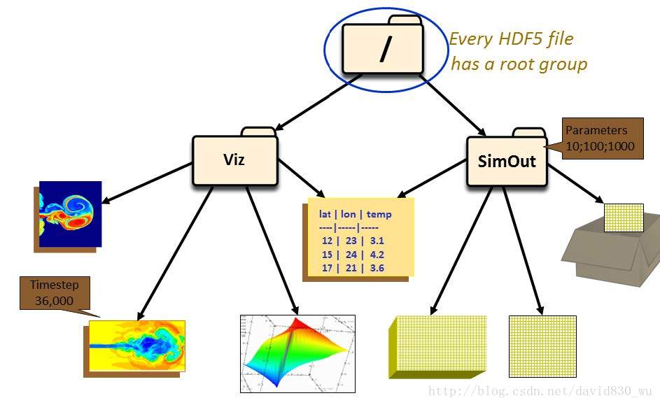
An HDF5 file contains:

• Groups: These are like directories or folders, used to organize your data. Groups can contain other groups, creating a hierarchy.
• Datasets: These are multidimensional arrays of a single data type, similar to a Julia Array. This is where your actual numerical data resides.
• Attributes: Small pieces of metadata (like numbers or strings) that can be attached to groups or datasets to describe them. Think of them as sticky notes for your data, perfect for storing parameters like "temperature=300K" or "LatticeSize=16".

The HDF5.jl package provides a high-level, Julian interface for interacting with HDF5 files.

Let's revisit our Hamiltonian example, but this time using HDF5.jl. Note how similar the code is to the jldopen syntax.

using HDF5
using LinearAlgebra




# Simulate some results (same as before)
H = rand(ComplexF64, 4, 4)
H = (H + H') / 2
E, V = eigen(H)
params = (N=4, coupling=0.5)

h5open("simulation_results.h5", "w") do file



    # Create a group for parameters
    g_params = create_group(file, "parameters")
    g_params["N"] = params.N
    g_params["coupling"] = params.coupling




    # Create a group for results
    g_results = create_group(file, "results")
    g_results["eigenvalues"] = E
    g_results["eigenvectors"] = V




    # Attach an attribute to the results group
    attrs(g_results)["description"] = "Eigen-decomposition of a random 4x4 Hermitian matrix."
end

The resulting .h5 file is now completely portable. You could open it in Python with h5py and find the exact same /parameters and /results structure. The Julia REPL itself provides a nice way to inspect the structure of these files.

JLD2 vs. HDF5: Which Should You Use?

You have two excellent tools at your disposal. Here’s a guide to choosing the right one for the job:

Use JLD2.jl when:

• You need to save arbitrary Julia objects. Your data will only be read by Julia, and you want to preserve custom structs, NamedTuples, or other complex types without any extra work.
• Simplicity and convenience are paramount. jldsave is incredibly easy to use for quick data dumps.
• You are checkpointing a long-running simulation. Saving the entire state of your Julia program is trivial with JLD2.

Use HDF5.jl when:

• You need to share data with colleagues who use Python, MATLAB, C++, etc.
• You are generating data for long-term archival. The language-agnostic nature of HDF5 makes it a much safer bet for future readability.
• You need to use external HDF5-compatible tools, such as the graphical HDFView application, to inspect your data.
• You are working with extremely large datasets and need to leverage advanced HDF5 features like parallel I/O, chunking, and compression schemes that are part of the HDF5 C library.

A common workflow in physics research is to use JLD2.jl for intermediate, development-stage data saving, and then write a script to convert the final, cleaned-up results into a well-structured HDF5 file for publication and sharing.

A Note on Tabular Data: JuliaDB

While JLD2 and HDF5 are perfect for array-based data, another class of data common in science is tabular data, where you have rows and columns, each with a specific meaning. For this, packages like DataFrames.jl are standard. For datasets that are too large to fit in memory, JuliaDB.jl provides a powerful solution. It can operate on data distributed across multiple processes and stored on disk.

Much like JLD2, JuliaDB has its own optimized binary format for saving and loading tables efficiently.

You are less likely to need JuliaDB for typical theoretical physics problems involving Hamiltonians and wavefunctions, but it's a valuable tool to be aware of if your work involves analyzing large, structured log files or other forms of tabular data.

Conclusion

You have now completed the first module and have a robust set of foundational skills for scientific computing in Julia. You can write efficient code, manipulate matrices, visualize your results, and now, reliably save and load your data for analysis and sharing.

Key Takeaways:

• Binary formats like JLD2 and HDF5 are essential for saving complex scientific data efficiently and robustly.
• JLD2.jl is the perfect tool for Julia-to-Julia data persistence, as it can flawlessly save and restore any Julia object.
• HDF5.jl is the industry standard for interoperable scientific data storage, allowing you to share data across different programming languages and tools.
• Both formats use a hierarchical model of groups and datasets, much like a filesystem, to keep your data organized.
• The choice between them depends on your primary goal: convenience and full Julia-type support (JLD2) versus interoperability and long-term archival (HDF5).

With this foundation laid, we are ready to move on. In the next module, Numerical Methods for Quantum Mechanics, we will begin applying these tools to solve physics problems. We will start by learning how to represent derivatives numerically and how to use Julia's powerful linear algebra capabilities to find the eigenvalues and eigenvectors of quantum systems.