Network Centrality Measures

What is Centrality?

"Importance" in a network is not a single concept. A person might be important because they have many friends, because they are a crucial link between different social circles, or because they are best positioned to spread news quickly. Centrality measures are designed to capture these different facets of structural importance.

Your background in operations research and statistics emphasizes quantifying system properties; think of centrality as a set of indices that quantify the structural properties of each node's position within the network graph.

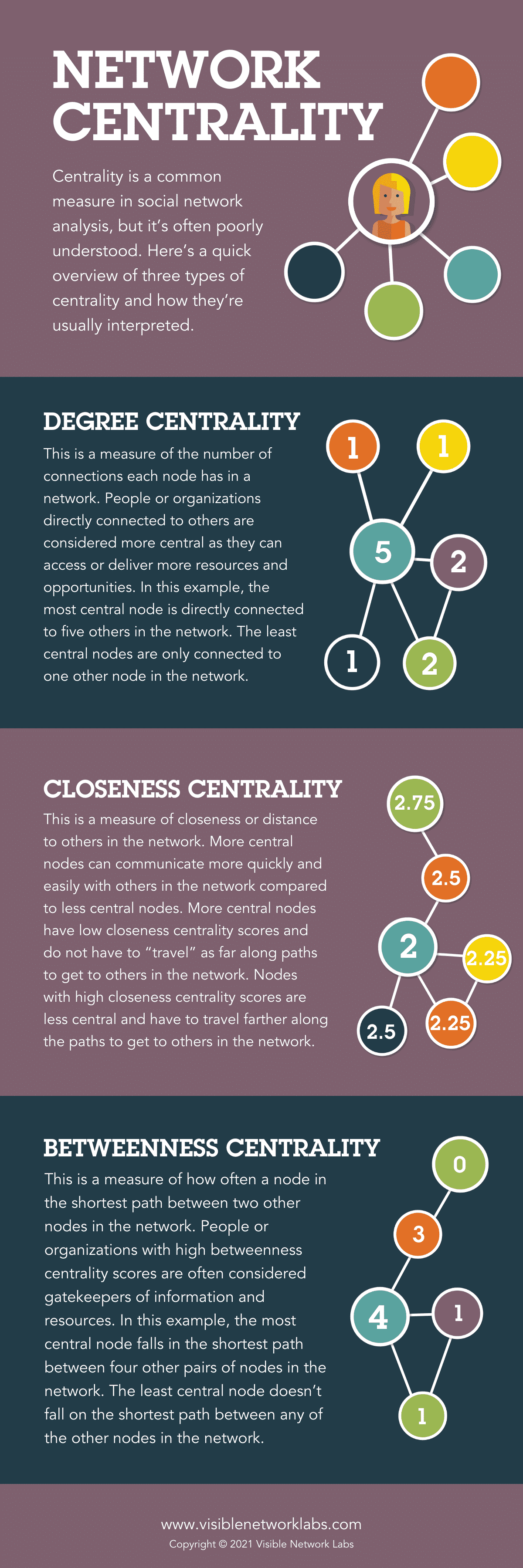
The following infographic provides a concise visual overview of the three measures we will explore today. It's a great reference point to keep in mind as we delve into each one.

Degree Centrality: The Measure of Direct Influence

Degree centrality is the most straightforward measure. As you'll recall from our last lesson, the degree of a node is simply the number of edges connected to it. In our context, this is the number of direct relationships a person has within the network.

A high degree centrality score indicates a node that is highly active or visible—a local hub. To understand the intuition and see how it's calculated, the following video provides a quick, clear explanation.

For a more formal definition, including the normalization formula, please refer to the following text.

Calculating Degree Centrality in a Vee

Let's apply this to our standard vee model, consisting of a hinge (H) and two non-hinge partners (P1 and P2). The graph has $n=3$ nodes.

1. Calculate Raw Degree:

   • Degree(H) = 2 (connected to P1 and P2)
   • Degree(P1) = 1 (connected to H)
   • Degree(P2) = 1 (connected to H)

2. Normalize the Degree: As the resources explain, normalization allows us to compare centrality scores across networks of different sizes. We divide by the maximum possible degree, which is $n-1$. Here, $n-1=2$.

   • Normalized Degree(H) = $2/(3-1)=1.0$
   • Normalized Degree(P1) = $1/(3-1)=0.5$
   • Normalized Degree(P2) = $1/(3-1)=0.5$

Interpretation: The hinge has the maximum possible degree centrality in this small network, formally capturing their role as the central hub of direct connections. The non-hinge partners are structurally identical and less central from a degree perspective.

Closeness Centrality: The Measure of Reach

Closeness centrality moves beyond direct ties to consider the entire network structure. It measures how easily a node can reach all other nodes in the network. A node has high closeness centrality if its average distance to all other nodes is short. Such nodes are in an excellent position to spread information efficiently.

The calculation is based on geodesic distance, which is simply the shortest path between two nodes. For a given node, you sum its geodesic distances to all other nodes, and then take the inverse.

Calculating Closeness Centrality in a Vee

1. Find all Geodesic Distances: Let $d(i,j)$ be the shortest path length between nodes $i$ and $j$.

   • $d(H,P1)=1$
   • $d(H,P2)=1$
   • $d(P1,P2)=2$ (The path is P1 → H → P2)

2. Sum Distances for Each Node:

   • Sum distances for H: $d(H,P1)+d(H,P2)=1+1=2$
   • Sum distances for P1: $d(P1,H)+d(P1,P2)=1+2=3$
   • Sum distances for P2: $d(P2,H)+d(P2,P1)=1+2=3$

3. Calculate Normalized Closeness: Using the formula $C_C^{\prime }(n_i)=(n-1)/{\sum }_{j=1}^{g}d(n_i,n_j)$:

   • Normalized Closeness(H) = $(3-1)/2=1.0$
   • Normalized Closeness(P1) = $(3-1)/3\approx 0.67$
   • Normalized Closeness(P2) = $(3-1)/3\approx 0.67$

Interpretation: Again, the hinge has the highest closeness score. This quantifies the idea that they are in the most efficient position to transmit information. News, plans, or emotional states originating from the hinge can reach both partners in a single step. For information to travel between P1 and P2, it takes two steps, making them less "close" to the network as a whole.

Betweenness Centrality: The Measure of Brokerage

Betweenness centrality captures a different, powerful form of importance: control over flow. It measures how often a node lies on the shortest path between other nodes. A node with high betweenness acts as a "bridge" or "gatekeeper," and can potentially control or filter what passes between others.

The calculation involves identifying all shortest paths between every pair of nodes and counting how many of those paths a given node falls upon.

Calculating Betweenness Centrality in a Vee

1. Identify All Pairs of Nodes and Their Shortest Paths:

   • Pair (P1, H): Shortest path is P1–H. No node is in between.
   • Pair (P2, H): Shortest path is P2–H. No node is in between.
   • Pair (P1, P2): The only shortest path is P1–H–P2. The hinge (H) lies on this path.

2. Calculate Betweenness Scores: We count, for each node, how many shortest paths it lies on.

   • Betweenness(H): Lies on the single shortest path between P1 and P2. Score = 1.
   • Betweenness(P1): Does not lie on any shortest paths between other nodes. Score = 0.
   • Betweenness(P2): Does not lie on any shortest paths between other nodes. Score = 0.

(Note on normalization: For a 3-node graph, the normalized scores are the same as the raw scores. The denominator $(g-1)(g-2)/2$ equals 1.)

Interpretation: This result is perhaps the most telling. The hinge is the only node with non-zero betweenness centrality. This starkly quantifies their role as a broker or gatekeeper. Any communication, resource flow, or negotiation between P1 and P2 must, by the structure of the vee, pass through H. This gives the hinge significant structural power and also places on them the responsibility of managing that flow.

Tying It All Together

Each centrality measure tells a different part of the story about the structure of a vee.

• Degree highlights the hinge as the most connected individual.
• Closeness highlights the hinge as the most efficient broadcaster.
• Betweenness highlights the hinge as the essential and exclusive broker.

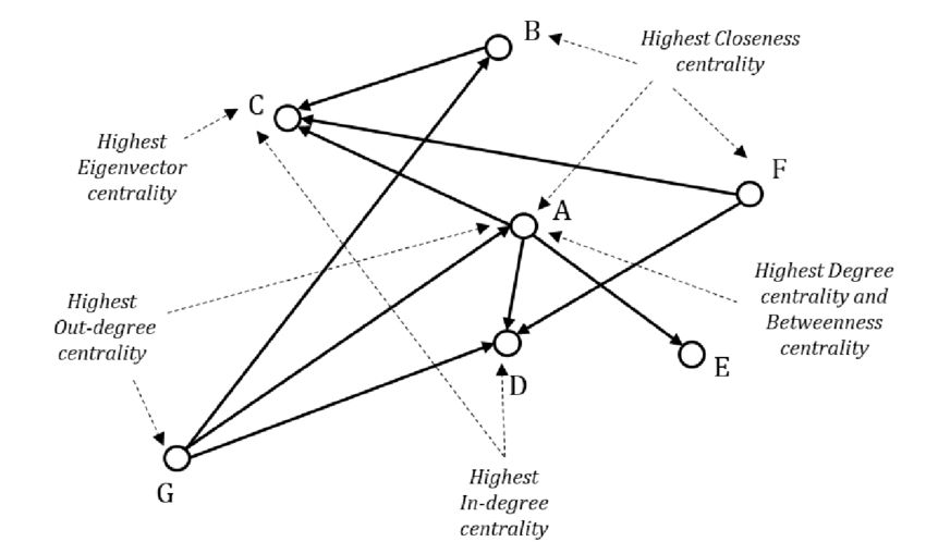
The image below shows a more complex, directed graph where different nodes excel on different measures. For instance, node A has high degree and betweenness (a hub and a broker), while node C has the highest eigenvector centrality (a different measure related to being connected to other important nodes), and node B has the highest closeness. This illustrates that these measures are not redundant and can reveal different kinds of importance in more complex networks.

Conclusion

In this lesson, you have learned to move from simply describing a vee network to analyzing the roles within it using quantitative measures. By computing and interpreting degree, closeness, and betweenness centrality, you can now formally articulate the structural position of each partner.

• Key Takeaways:
  • Degree Centrality measures direct connections (popularity/activity). In a vee, the hinge has a score of 1.0, while partners have 0.5.
  • Closeness Centrality measures efficiency in reaching others (information spreading). In a vee, the hinge has a score of 1.0, while partners have ~0.67.
  • Betweenness Centrality measures control over information flow (brokerage). In a vee, the hinge has a score of 1.0, while partners have 0.
  • While the hinge consistently scores highest, each measure illuminates a different facet of their central role: being a hub, an efficient broadcaster, and an exclusive gatekeeper.

Preview of the next lesson:
The concept of betweenness centrality, which identifies nodes as bridges, is a perfect gateway to our next topic. We will delve deeper into the role of the hinge as a broker by exploring the concepts of structural holes and brokerage positions. You will learn how the "gap" between the two non-hinge partners creates both opportunities and constraints for the hinge, further enriching our understanding of the vee's internal dynamics.