Introduction
Welcome to the first lesson of our module on Statistical Process Control (SPC). In our previous module, we concluded the "Improve" phase of DMAIC by successfully running a pilot test to validate our proposed solution. We now have a data-driven confirmation that our changes work and deliver the expected benefits. The challenge now shifts from improving the process to controlling it, ensuring that our hard-won gains are sustained over time.
This lesson marks our entry into the "Control" phase. The primary tool we'll use to monitor and maintain process stability is the control chart. However, there isn't a one-size-fits-all control chart. Using the wrong one can lead to false alarms or, worse, failing to detect a problem when one exists.
Therefore, our focus for this lesson is on the learning outcome: Select the appropriate control chart based on data type (X-bar/R, X-bar/S, I-MR, p, np, c, u). We will establish a clear decision-making framework, so you can confidently choose the most powerful chart for any given manufacturing scenario. This foundational skill is essential before we move on to building and interpreting these charts in the next lesson.
1. The First Decision: Variable vs. Attribute Data
The most fundamental step in selecting a control chart is to identify the type of data you are working with. All process data can be classified into one of two categories: variable or attribute.
-
Variable Data (or continuous data) are measurements taken on a continuous scale. These can be broken down into finer and finer increments. Think of things you measure.
- Examples: Length in millimeters, weight in grams, temperature in Celsius, pressure in PSI, cycle time in seconds.
-
Attribute Data (or discrete data) are counts of items or characteristics. These are whole numbers and cannot be broken down into smaller parts. Think of things you count.
- Examples: The number of non-conforming parts, a pass/fail classification, the number of scratches on a car door, the number of complaints in a day.
Getting this distinction right is the first and most critical gate in the selection process. The flowchart below will be our guide for this entire lesson. Notice how the first split is between "Variable Data" and "Attribute Data."
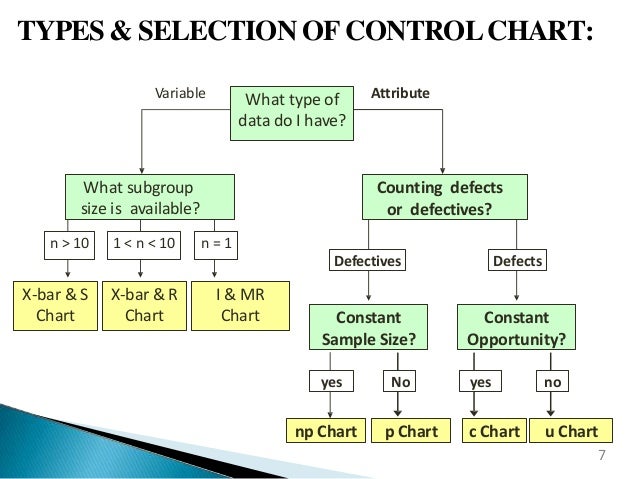
2. Control Charts for Variable (Continuous) Data
When you have measurement data, the next question to ask is about your subgroup size (n). A subgroup is a small sample of items collected from the process at a single point in time. The way you sample is crucial; this practice, known as rational subgrouping, aims to capture the natural, common-cause variation within the subgroup, making it easier to see special-cause variation between subgroups over time.
The choice of control chart for variable data is determined by the size of these subgroups.
A Practical Guide to Selecting the Right Control Chart
The following guide from InfinityQS provides an excellent, practical overview of selecting the three core control charts for variable data based on subgroup size.
Please read Part 2, "The Three Core Variables Charts: Using Sample Size to Determine Core Chart Type" (pages 6-9). As you read, focus on the rationale for using each chart based on the sample size n.
Let's summarize the key decision points from the reading.
Subgroup Size n = 1: Individuals and Moving Range (I-MR) Chart
You use an I-MR chart when you only have a single observation at each time point. This is common in several manufacturing scenarios:
- Processes with long cycle times where taking multiple samples is impractical.
- Automated data collection that provides one reading per interval (e.g., furnace temperature every 5 minutes).
- Destructive testing (e.g., tensile strength tests).
- Homogeneous batches (e.g., chemicals, paint) where multiple samples from the same batch would only reflect measurement error, not process variation.
The I-MR chart consists of two plots:
- The Individuals (I) chart plots the individual measurement values.
- The Moving Range (MR) chart plots the absolute difference between consecutive measurements, which provides an estimate of process variability.
Subgroup Size 2 ≤ n ≤ 9: X-bar and Range (X-bar & R) Chart
This is one of the most common control charts. It's used when you can collect small subgroups (typically 3 to 5 items) at regular intervals.
- The X-bar ( ) chart plots the average of each subgroup. It monitors the central tendency of the process.
- The Range (R) chart plots the range (Maximum - Minimum value) within each subgroup. It monitors the short-term variability of the process.
For small subgroups, the range is a simple yet effective way to estimate process variation.
Subgroup Size n ≥ 10: X-bar and Standard Deviation (X-bar & S) Chart
When you can collect larger subgroups, the X-bar & S chart is more statistically powerful than the X-bar & R chart. This is because the standard deviation uses all the data points in the subgroup to calculate variation, whereas the range only uses the highest and lowest values.
- The X-bar ( ) chart is the same as before, plotting subgroup averages.
- The Standard Deviation (S) chart plots the standard deviation of each subgroup. It provides a more robust and sensitive measure of process variability than the range for larger sample sizes.
To see these charts explained with simple examples, watch the following video segments.
Control Charts simply explained - Statistical process control - Xbar-R Chart, I-MR Chart,...
This video from numiqo provides a quick visual explanation of the X-bar & R and I-MR charts.
Watch the following two segments: 01:00 - 05:05: This covers the X-bar & R chart. Focus on the concept of plotting subgroup means and ranges over time. 05:05 - 06:25: This explains the I-MR chart and highlights the key difference from the X-bar chart (having only one observation per time point).
3. Control Charts for Attribute (Discrete) Data
Now let's move to the other side of our flowchart. When you are counting things rather than measuring them, you are dealing with attribute data. The selection process here involves two questions:
- Are you counting defective units or the number of defects?
- Is your sample size (or area of opportunity) constant or variable with each sample?
The distinction between "defectives" and "defects" is crucial. Let's dive into that first.
Attribute Data Control Chart Examples!! How to select/create the P, NP, C and U Charts
The following video from CQE Academy does an exceptional job of clarifying the difference between 'defectives' and 'defects' and how this choice, along with sample size, dictates which attribute chart to use.
Please watch from the beginning until 03:57. Focus on: The definition of a 'defective unit' (a pass/fail item). The definition of a 'defect' (a flaw, where one unit can have multiple flaws). How these definitions, combined with sample size, map to the four main attribute charts (p, np, c, u).
As the video explained:
- A defective is a unit that fails to meet specifications. It's a binary, pass/fail judgment. We count the number of bad parts. This type of data follows a binomial distribution.
- A defect is a specific flaw or nonconformity on a unit. A single unit can have multiple defects. We count the number of flaws. This type of data follows a Poisson distribution.
With this understanding, we can now select the correct attribute chart.
Counting Defectives (Pass/Fail Classification)
- np-Chart: Use when you are counting the number of defective units and your sample size is constant for every subgroup. For example, you inspect 100 units every hour and plot the number that failed.
- p-Chart: Use when you are counting defective units but your sample size is variable. The chart plots the proportion (or percentage) of defective units in each subgroup (). For example, you inspect the full output of a line each day, and the daily production volume varies.
Counting Defects (Flaws)
- c-Chart: Use when you are counting the number of defects and your area of opportunity is constant. For example, you count the number of paint blemishes on car hoods, and each hood is the same size. You plot the raw count of defects per hood.
- u-Chart: Use when you are counting the number of defects but your area of opportunity is variable. The chart plots the rate of defects (). For example, you inspect rolls of fabric for flaws, but the rolls come in different lengths. You would plot the number of flaws per square meter.
To reinforce your understanding, the following video walks through examples for each of the four attribute charts.
Control Charts simply explained - Statistical process control - Xbar-R Chart, I-MR Chart,...
This video from numiqo provides short, practical examples for each of the four attribute charts.
Please watch from 07:11 to 10:42. For each chart type (np, p, c, u), focus on the type of data being counted and whether the sample size is constant or variable.
Summary of Control Chart Selection
You now have a complete framework for selecting the most common types of control charts. Let's consolidate this into a quick-reference table.
| Data Type | What are you tracking? | Subgroup/Opportunity Size | Chart to Use |
|---|---|---|---|
| Variable | Individual measurements | n = 1 | I-MR |
| (Continuous) | Subgroup averages & variability | 2 ≤ n ≤ 9 | X-bar & R |
| Subgroup averages & variability | n ≥ 10 | X-bar & S | |
| Attribute | Number of defective units | Constant | np-Chart |
| (Discrete) | Proportion of defective units | Variable | p-Chart |
| Number of defects | Constant | c-Chart | |
| Rate of defects per unit | Variable | u-Chart |
This decision logic is the first and most critical step in implementing Statistical Process Control.
Conclusion
In this lesson, we established the systematic process for selecting the correct control chart. We started with the fundamental distinction between variable and attribute data and then explored the specific decision criteria for each data type. For an experienced Industrial Engineer like yourself, mastering this selection process formalizes a key Green Belt skill and provides the foundation for the more advanced control strategies you'll encounter at the Black Belt level.
Key Takeaways:
- Control chart selection begins with identifying your data as either variable (measured) or attribute (counted).
- For variable data, the choice depends on the subgroup size: I-MR for individuals (n=1), X-bar & R for small subgroups (2-9), and X-bar & S for large subgroups (≥10).
- For attribute data, the choice depends on whether you are counting defectives (bad parts) or defects (flaws), and whether the sample size or area of opportunity is constant or variable.
- This leads to four attribute charts: p-chart (variable sample, defectives), np-chart (constant sample, defectives), u-chart (variable opportunity, defects), and c-chart (constant opportunity, defects).
Preview of the Next Lesson:
Now that you know how to select the right tool for the job, our next lesson will focus on how to use it. We will address the learning outcome: Construct and interpret control charts for ongoing manufacturing process monitoring. We'll take a practical scenario, apply the selection logic from today, build the corresponding chart, and learn how to interpret the patterns it reveals about our process.