Welcome. This is the first lesson in the Python DSA interview track, which will build the core patterns needed to reason about and implement interview solutions in Python. We begin with a skill that underlies every later choice: looking at a short function and stating how its runtime and memory use scale as the input grows.
For an ML engineer, this is also a practical systems skill. A data-processing step that is harmless on one hour of audio can become a bottleneck across millions of utterances; an apparently simple nested comparison can dominate an evaluation pipeline. In interviews, however, the goal is more disciplined: identify the input size, trace the operations that scale with it, and state a defensible time and space complexity.
By the end of this lesson, you should be able to analyze typical Python loops, nested loops, halving loops, allocations, and short recursive functions using Big-O notation.
Complexity is about growth, not stopwatch time
Suppose a function receives a list samples of length . The value is the input size. We ask:
If becomes much larger, how does the amount of work grow?
We usually model runtime as a count of elementary operations rather than milliseconds. Wall-clock time depends on hardware, Python version, cache behavior, and implementation details. Big-O deliberately ignores those details so that it captures the part that matters when data scales.
Consider:
def mean_energy(samples):
    total = 0.0

    for x in samples:
        total += x * x

    return total / len(samples)
The loop visits every sample once. If there are samples, it performs roughly loop-body updates, plus a fixed amount of setup and return work:
where and are constants. We write its running time as:
This is linear time. Doubling the number of samples roughly doubles the work.
Now contrast it with a function that compares every frame with every frame:
def total_pair_distance(features):
    total = 0.0
    n = len(features)

    for i in range(n):
        for j in range(n):
            total += abs(features[i] - features[j])

    return total
For every one of the outer-loop iterations, the inner loop performs iterations. The loop body therefore runs:
times, so time complexity is:
That distinction is important: a pairwise operation over 1,000 items is about one million comparisons; over 100,000 items, it is about ten billion.
Time & Space Complexity - Big O Notation - DSA Course in Python Lecture 1
Watch “Time & Space Complexity - Big O Notation - DSA Course in Python Lecture 1” by Greg Hogg for a concise visual introduction to linear versus quadratic work, auxiliary space, and the simplification rules used in interview answers.
Watch linear and quadratic to visualize why processing items once differs fundamentally from generating pairs. Then watch space complexity, focusing on the difference between creating a new output list and modifying an existing list. Finish with simplification rules and common hierarchy. Notice that fixed constants and lower-order terms are dropped because they do not change long-run growth.
The common growth classes worth recognizing immediately are:
| Complexity | Name | Typical signal in code |
|---|---|---|
| constant | fixed number of operations | |
| logarithmic | input is repeatedly halved or otherwise reduced by a constant factor | |
| linear | one pass over an input | |
| log-linear | efficient comparison sorting, divide-and-conquer work | |
| quadratic | all pairs; two dependent nested loops | |
| exponential | recursively branch into multiple subproblems without caching | |
| factorial | enumerate permutations or every ordering |
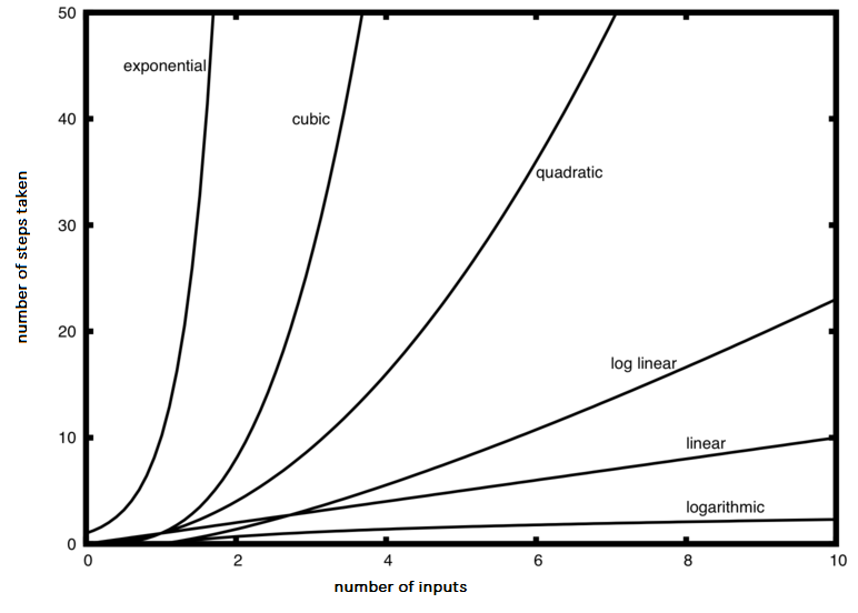
The plotted range is small, but the trend is the point. At tiny , implementation constants can matter more than asymptotic class. At production or interview-scale , the growth rate usually decides whether an approach is viable.
What Big-O simplifies—and what it does not
Big-O describes an asymptotic upper bound: beyond some sufficiently large input size, the work is bounded above by a constant multiple of a function. In interview conversation, saying “the complexity is ” generally means “ is the tightest standard upper bound we have identified.”
Two simplification rules do most of the work.
Drop constant multipliers
If a function makes three complete passes through a list, its operation count may be approximately . Its Big-O time is still:
Likewise, is . It may be significantly slower in practice than , but both scale linearly.
Keep only the dominant term
For:
the quadratic term eventually dominates:
Do not apply these rules before understanding the structure. First write the work contributed by each block; then simplify.
A useful interview habit is to state your reasoning in this order:
- “The first loop runs times.”
- “The second loop also runs times, but it is nested.”
- “So the body executes times.”
- “Therefore the time complexity is .”
That makes your answer auditable rather than a guess based solely on the number of for keywords.
A reliable procedure for analyzing short Python functions
Use this six-step process.
1. Define the input-size variables
A single list usually has length :
def f(items):
    ...
If a function receives two independently sized inputs, use separate variables:
def compare(a, b):
    ...
Let:
Do not assume both have equal length unless the function contract guarantees it.
2. Ignore fixed-size work initially
Assignments, arithmetic on scalar variables, comparisons, and indexing are usually treated as constant-time operations under the normal algorithm-analysis model.
For example:
first = values[0]
limit = 10
return first + limit
is time, assuming values is nonempty. It does not matter whether the list has 10 items or 10 million: the code performs a fixed amount of work.
A fixed count is still constant:
for _ in range(100_000):
    update_state()
This is with respect to input size. It may be a poor engineering choice because 100,000 operations are substantial, but the count does not grow when the caller supplies more input.
3. Add sequential blocks
def summarize(values):
    total = 0
    for x in values:
        total += x

    maximum = values[0]
    for x in values:
        if x > maximum:
            maximum = x

    return total, maximum
The first loop costs , and the second costs :
Thus:
Sequential loops add; they do not multiply.
4. Multiply nested dependent loops
def print_pairs(values):
    for x in values:
        for y in values:
            print(x, y)
For each of choices of x, the inner loop visits values of y:
So time is .
If the collections differ:
def cross_score(queries, candidates):
    for query in queries:
        for candidate in candidates:
            score(query, candidate)
then the correct answer is:
not automatically . It becomes only if both inputs are known to have the same size .
5. Check whether a loop shrinks the problem
def reduction_steps(n):
    steps = 0

    while n > 1:
        n //= 2
        steps += 1

    return steps
The successive values are approximately:
After iterations, the value is about . The loop ends near 1, so:
which implies:
Therefore the time complexity is:
The base of the logarithm is not written in Big-O because changing bases only introduces a constant factor.
6. Count extra memory separately
After time, ask: what extra storage does the function allocate as the input grows?
Do not count the input itself when reporting auxiliary space. Count new lists, dictionaries, sets, copies, recursion frames, and other storage created by the algorithm.
Time complexity and auxiliary space are different questions
Return to the energy example:
def mean_energy(samples):
    total = 0.0

    for x in samples:
        total += x * x

    return total / len(samples)
It has:
- Time: , because every sample is visited.
- Auxiliary space: , because
totalandxare a fixed number of scalar variables.
Now consider a function that creates a separate output:
def square_copy(values):
    result = []

    for x in values:
        result.append(x * x)

    return result
It also visits each value once:
But result grows to contain elements:
If you modify a mutable input in place instead:
def square_in_place(values):
    for i in range(len(values)):
        values[i] = values[i] * values[i]
then:
- Time:
- Auxiliary space:
The input list already exists; the function only uses a fixed number of extra variables.
The output-space convention
Interviewers differ on whether the returned output should count as space. Avoid ambiguity by stating the convention:
“The auxiliary space is , excluding the output. If we count the returned list, total additional storage is .”
For square_copy, that distinction is especially important. For print_pairs, materializing all pairs in a list would require output space—because there are pairs to store.
Code patterns that reward careful counting
The next video works through code examples similar to the ones you will see in Python interviews. Pay particular attention to the distinction between sequential and nested loops, and to the fact that a loop bounded by a fixed constant does not add another factor.
Big O Notation - Code Examples
Watch “Big O Notation - Code Examples” by Keep On Coding for a code-first walkthrough of sequential loops, nested loops, and separate input dimensions.
Watch sequential loops to reinforce why two passes are O(n), not O(n^2). Then watch nested loops for the multiplication argument behind O(n^2). Finish with different dimensions; the key point is that loops over separate arrays should be expressed as O(mn) when their sizes are independent.
Here are three cases where simply “counting loops” gives the wrong answer.
Triangular nested loops are still quadratic
def unique_pairs(values):
    pairs = []

    for i in range(len(values)):
        for j in range(i + 1, len(values)):
            pairs.append((values[i], values[j]))

    return pairs
The inner loop does not always run times:
- for
i = 0, it runs times; - for
i = 1, it runs times; - eventually it runs 0 times.
The total work is:
After dropping constants and lower-order terms:
Avoid saying “there are two loops, therefore .” Instead, count iterations. It happens to be quadratic here, but for a reason.
A break changes best case, not necessarily worst case
def contains_negative(values):
    for x in values:
        if x < 0:
            return True
    return False
- Best case: the first value is negative, so .
- Worst case: no negative value exists, or it occurs last, so .
Unless an interviewer asks for best-case behavior, report the usual worst-case complexity:
You can add: “Best case is because of the early return.”
Recursion may consume stack space
def countdown(n):
    if n == 0:
        return
    countdown(n - 1)
There is one recursive call per decrement:
At the deepest point, there are active calls on Python’s call stack:
A recursive function may have linear time but nonconstant space even if it does not allocate an explicit list.
Python-specific details worth remembering
Big-O analyzes the code you actually write, not just the loops you see. These operations frequently matter:
| Python operation | Typical complexity | Why it matters |
|---|---|---|
len(values) |
Python sequences store their length. | |
values[i] for a list |
Lists support direct indexed access. | |
for x in values |
total | The iterator visits each element once. |
list.append(x) |
amortized | Resizing occasionally costs more, but average append cost is constant. |
x in some_list |
Membership scans until it finds x or reaches the end. |
|
values[:] |
time and space | A slice copy allocates a new list. |
sorted(values) |
time | Sorting performs more than a single pass and returns a new list. |
range(n) |
space | In modern Python, range represents a progression lazily rather than creating a full list. |
A caveat for later: dictionary and set lookup are typically treated as expected , but their behavior rests on hashing assumptions. The next lesson will use that fact carefully for frequency-counting problems.
A compact interview-answer template
When asked for the complexity of a function, give both a conclusion and its basis:
“Let be the number of input elements. The outer loop runs times, and the inner loop runs times for each outer iteration, so the body executes times. Time is . The function only stores scalar counters, so auxiliary space is .”
For a function returning a list, add the output convention explicitly:
“Time is . Auxiliary space excluding the returned output is ; including the output list, it is .”
Before committing to an answer, run this mental checklist:
- What is , and are there independent sizes such as and ?
- Are loops sequential (add) or nested (often multiply)?
- Does a loop reduce the remaining work by a factor, suggesting ?
- Does an early exit change the best case only?
- What new storage grows with input size?
- Am I reporting worst-case time unless a different case was requested?
Key takeaways
Big-O is a language for describing how resource use grows with input size. Fixed work is ; one full traversal is generally ; dependent nested traversals are often ; and repeated halving yields .
For short Python functions, first identify the size variables, then add sequential costs, multiply genuinely nested costs, simplify to the dominant term, and separately count additional memory. Be precise about best versus worst case and about whether reported space includes a materialized output.
Next, you will apply this analysis while using Python dictionaries and sets to solve a frequency-counting problem—an important pattern where a small amount of extra space can replace a costly nested-loop search.