Cosmological Redshift and the Hubble-Lemaître Law

Hello! Welcome to the next lesson in our journey through cosmology.

In our last session, we solved the Friedmann equations for idealized universes, finding that the scale factor $a (t)$ evolves as a power law or an exponential function depending on whether matter, radiation, or vacuum energy dominates. We now have a dynamical model for how the universe expands.

Today, we will connect this abstract expansion to a cornerstone of observational cosmology. Our learning outcome is to define cosmological redshift and derive the Hubble-Lemaître law. We will demonstrate how the observed redshift of distant galaxies is a direct and profound consequence of the evolving spacetime described by $a (t)$ , and how this leads to the famous law relating recessional velocity to distance for nearby objects.

1. The Physical Origin of Cosmological Redshift

At its heart, cosmological redshift is the stretching of light waves as they travel through expanding space. As a photon propagates from a distant galaxy to us, the universe expands. The wavelength of the photon, being a physical length, is stretched along with the fabric of spacetime. A wave emitted with wavelength $λ_{e}$ arrives with a longer wavelength $λ_{o}$ .

This intuitive picture is backed by a rigorous derivation from the FRW metric, which precisely describes this expanding spacetime.

Rigorous Derivation

Let's trace the path of a light wave from a distant source to an observer. Light travels along null geodesics, where $d s^{2} = 0$ . In the FRW metric, for a photon traveling radially ( $d θ = d ϕ = 0$ ) from a source at comoving coordinate $r_{e}$ to an observer at the origin ( $r = 0$ ), this condition becomes:

d s^{2} = - c^{2} d t^{2} + a (t)^{2} \frac{d r ^{2}}{1 - k r ^{2}} = 0

Rearranging for an incoming photon gives:

\frac{c d t}{a ( t )} = - \frac{d r}{1 - k r ^{2}}

Now, consider two successive wave crests emitted from the source.

Crest 1 is emitted at time $t_{e}$ and observed at time $t_{o}$ .
Crest 2 is emitted a short time later, at $t_{e} + δ t_{e}$ , and observed at $t_{o} + δ t_{o}$ .

We can integrate the geodesic equation for each crest's journey. Since the comoving coordinates of the source and observer are fixed, the spatial integral is the same for both:

\int_{t_{e}}^{t_{o}} \frac{c d t}{a ( t )} = \int_{0}^{r_{e}} \frac{d r}{1 - k r ^{2}} (for Crest 1)

\int_{t_{e} + δ t_{e}}^{t_{o} + δ t_{o}} \frac{c d t}{a ( t )} = \int_{0}^{r_{e}} \frac{d r}{1 - k r ^{2}} (for Crest 2)

Equating the two time integrals, we get:

\int_{t_{e}}^{t_{o}} \frac{d t}{a ( t )} = \int_{t_{e} + δ t_{e}}^{t_{o} + δ t_{o}} \frac{d t}{a ( t )}

We can split the integrals and cancel the common overlapping interval $\int_{t_{e} + δ t_{e}}^{t_{o}}$ , which leaves:

\int_{t_{e}}^{t_{e} + δ t_{e}} \frac{d t}{a ( t )} = \int_{t_{o}}^{t_{o} + δ t_{o}} \frac{d t}{a ( t )}

Since the time intervals $δ t_{e}$ and $δ t_{o}$ (the period of the light wave) are infinitesimally short compared to cosmological timescales, we can treat $a (t)$ as constant over each integration. This simplifies the equation to:

\frac{δ t _{e}}{a ( t _{e} )} \approx \frac{δ t _{o}}{a ( t _{o} )}

The period of a wave ( $δ t$ ) is related to its wavelength ( $λ$ ) by $λ = cδ t$ . Substituting this in, we arrive at the fundamental result:

\frac{λ _{o}}{c a ( t _{o} )} = \frac{λ _{e}}{c a ( t _{e} )} ⟹ \frac{λ _{o}}{λ _{e}} = \frac{a ( t _{o} )}{a ( t _{e} )}

The redshift parameter, $z$ , is defined as the fractional increase in wavelength:

z \equiv \frac{λ _{o} - λ _{e}}{λ _{e}} = \frac{λ _{o}}{λ _{e}} - 1

Combining these gives the cornerstone equation of observational cosmology:

1 + z = \frac{a ( t _{o} )}{a ( t _{e} )}

This beautiful equation tells us that by measuring the redshift of a distant object, we are directly measuring how much the universe has expanded since the light was emitted.

Cosmological Redshift Derivation — This diagram succinctly summarizes the mathematical steps we just took to relate the observed and emitted wavelengths to the scale factor at the times of observation and emission.

The following resources provide this same derivation and offer alternative perspectives.

The Friedmann–Lemaˆıtre–Robertson–Walker model

For a clear and formal derivation, please read the following section from the lecture notes by Syksy Räsänen.

Please read section 3.1.3, 'Redshift'. It follows the exact logic we've just discussed, culminating in Equation (3.17).

Relativity 110d: Cosmology - FLRW Geodesics, Cosmological Redshift, Horizons, Comoving Coordinates

For a more intuitive approach that complements the formal derivation, the eigenchris channel offers an excellent explanation. It focuses on the idea that the coordinate distance between wave crests remains constant, while the physical distance stretches with the scale factor.

Watch the segment from 10:56 to 16:28. Notice how he arrives at the same conclusion (\lambda_o/\lambda_e = a_o/a_e) using a conceptual argument about coordinate vs. physical distance.

Test your understanding!

We observe a quasar at a redshift of $z = 7$ . We know from the previous lesson that during the matter-dominated era, the universe expands as $a (t) \propto t^{2/3}$ . Assuming the light was emitted during this era and we observe it today (also in this era for the sake of this problem), by what factor was the universe younger when the light was emitted compared to its age today?

Show answer

First, relate the scale factors using the redshift: $1 + z = \frac{a ( t _{o} )}{a ( t _{e} )} ⟹ \frac{a ( t _{o} )}{a ( t _{e} )} = 1 + 7 = 8$
Next, use the expansion law $a (t) = C t^{2/3}$ for a matter-dominated universe: $\frac{a ( t _{o} )}{a ( t _{e} )} = \frac{C t _{o}^{2/3}}{C t _{e}^{2/3}} = (\frac{t _{o}}{t _{e}})^{2/3}$
Equate the two expressions: $(\frac{t _{o}}{t _{e}})^{2/3} = 8$
Solve for the ratio of the ages $t_{o} / t_{e}$ : $\frac{t _{o}}{t _{e}} = 8^{3/2} = (8)^{3} = (22)^{3} = 8 \cdot 22 = 162 \approx 22.6$ So, the universe was about 22.6 times younger when the light was emitted. The age at emission was $t_{e} = t_{o} / (162)$ .

2. The Hubble-Lemaître Law as a Low-Redshift Limit

The Hubble-Lemaître law, $v = H_{0} d$ , states that the recessional velocity $v$ of a galaxy is proportional to its proper distance $d$ , with the constant of proportionality being the Hubble constant $H_{0}$ . This is not a new fundamental law, but rather the low-redshift approximation of our cosmological redshift formula.

Let's consider an object that is relatively nearby. This means the light from it was emitted at a time $t_{e}$ that is not too far in the past. The lookback time, $Δ t = t_{o} - t_{e}$ , is small. We can perform a first-order Taylor expansion of $a (t_{e})$ around the present time $t_{o}$ :

a (t_{e}) = a (t_{o} - Δ t) \approx a (t_{o}) - a ˙ (t_{o}) Δ t

Now substitute this into our redshift equation:

1 + z = \frac{a ( t _{o} )}{a ( t _{e} )} \approx \frac{a ( t _{o} )}{a ( t _{o} ) - a ˙ ( t _{o} ) Δ t} = \frac{1}{1 - \frac{a ˙ ( t _{o} )}{a ( t _{o} )} Δ t}

We recognize the term $\frac{a ˙ ( t _{o} )}{a ( t _{o} )}$ as the definition of the Hubble parameter at the present time, $H_{0}$ . For small $x$ , the approximation $(1 - x)^{- 1} \approx 1 + x$ is valid. Applying this gives:

1 + z \approx 1 + H_{0} Δ t ⟹ z \approx H_{0} Δ t

For small distances in an expanding universe, the proper distance $d$ is simply the light travel time multiplied by the speed of light, $d \approx c Δ t$ . Substituting $Δ t \approx d / c$ , we get:

z \approx \frac{H _{0} d}{c}

Finally, for low velocities, the special relativistic Doppler effect gives a redshift of $z \approx v / c$ . Equating these two expressions for $z$ gives us the famous law:

\frac{v}{c} \approx \frac{H _{0} d}{c} ⟹ v \approx H_{0} d

This derivation shows that the linear relationship observed by Hubble and Lemaître is a direct and necessary consequence of the expansion of spacetime in General Relativity.

The Friedmann–Lemaˆıtre–Robertson–Walker model

The lecture notes from the University of Helsinki confirm this result concisely.

Please read the brief section 3.1.8, 'The Hubble law'. It states that for small redshifts (z \ll 1), the different cosmological distance measures all agree and lead to the linear law we just derived.

3. Cosmological vs. Doppler Redshift

It's crucial to understand the physical distinction between cosmological redshift and the more familiar Doppler and gravitational redshifts.

Doppler Redshift: Arises from the peculiar motion of an object through space, relative to an observer.
Gravitational Redshift: Arises when light loses energy climbing out of a gravitational potential well.
Cosmological Redshift: Arises from the expansion of space itself, which stretches the wavelength of light as it propagates.

For nearby galaxies ( $z ≪ 1$ ), the Hubble-Lemaître law $v \approx H_{0} d$ looks like a Doppler shift, and it's often described in terms of a "recession velocity". However, this is just a low-velocity analogy. The underlying cause is the expansion of the universe, not galaxies flying away from us through static space.

For distant objects with high redshift, this distinction becomes critical. The recessional velocity $v = H_{0} d$ can, and does, exceed the speed of light $c$ . This does not violate special relativity, because it is the space between objects that is expanding; no object is moving locally through space faster than light.

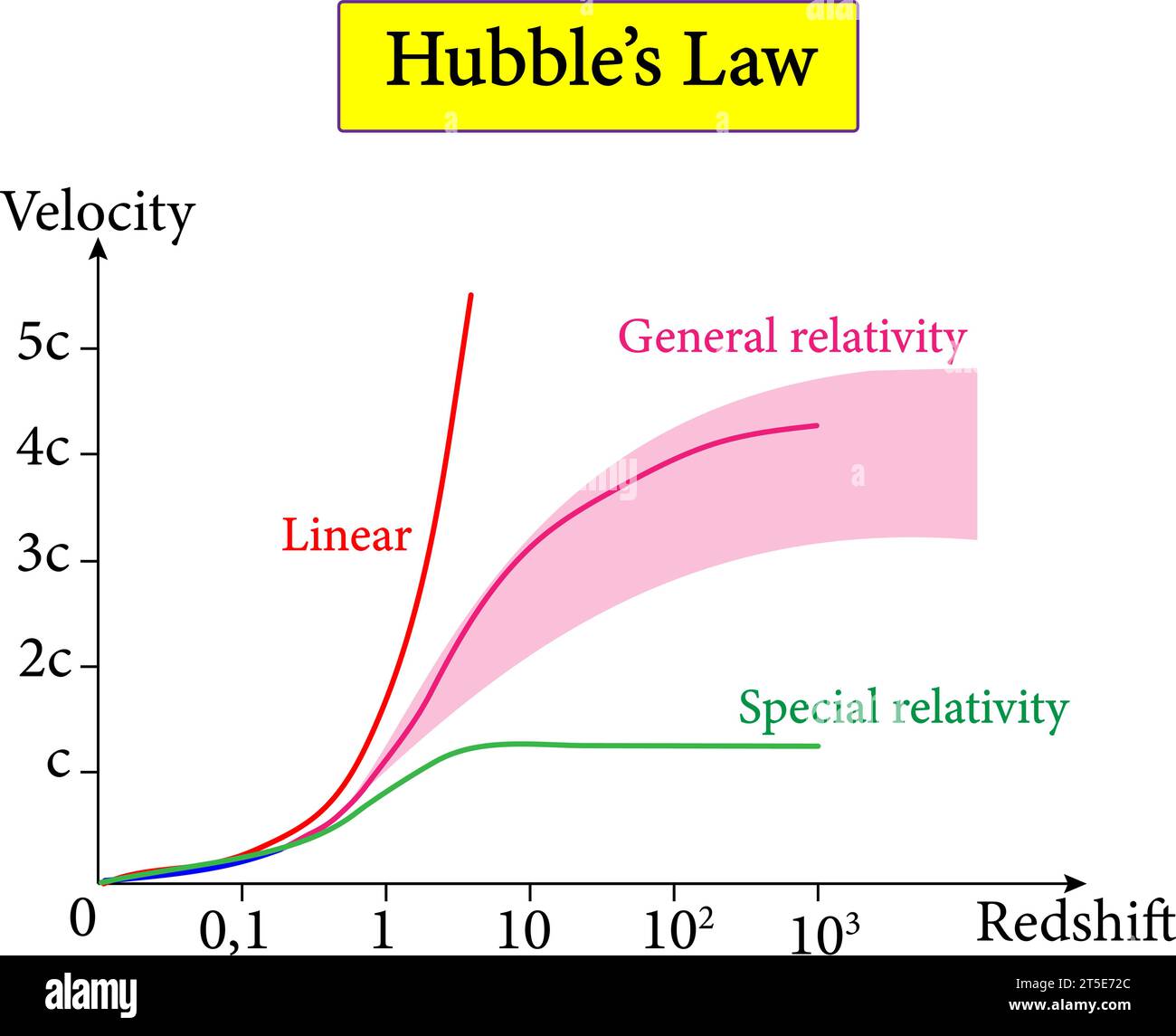
Hubble's Law: Velocity vs. Redshift in Different Relativistic Regimes — This graph shows the relationship between recessional velocity and redshift. The simple linear law (naive Doppler interpretation) quickly and incorrectly exceeds 'c'. Special Relativity forbids any object from reaching 'c'. General Relativity (the cosmological model) shows that the recessional velocity, due to the expansion of space itself, can indeed exceed 'c' at high redshifts.

This topic, which connects the formalisms of SR and GR in a cosmological context, is quite subtle. The following video provides a very clear and high-level discussion that your physics background will allow you to appreciate fully.

5. Cosmological Redshift and the Dynamics of Homogeneous Expansion, Part I

Professor Alan Guth's lecture from MIT OpenCourseWare offers a fantastic discussion comparing the SR Doppler shift with the cosmological redshift calculation.

Please watch the segment from 17:43 to 25:07. Professor Guth explains why the cosmological calculation is more powerful (it includes gravity via a(t)) and how the two calculations use fundamentally different variables (cosmic time vs. inertial frame time).

Conclusion

In this lesson, we have forged the crucial link between the theoretical dynamics of the FRW metric and a key cosmological observable.

Key Takeaways:

Cosmological redshift is caused by the expansion of space stretching the wavelength of light.
The redshift $z$ is directly related to the change in the universe's scale factor between emission ( $a_{e}$ ) and observation ( $a_{o}$ ) by the fundamental formula: $1 + z = a_{o} / a_{e}$ .
The Hubble-Lemaître law, $v \approx H_{0} d$ , is the low-redshift ( $z ≪ 1$ ) approximation of this general relativistic effect.
The "recession velocity" in the Hubble-Lemaître law is not a local velocity through space and can exceed the speed of light for distant objects.

Preview of Next Lesson:

We have derived $v \approx H_{0} d$ . But how do we actually measure the distance $d$ to a faraway galaxy? In an expanding and potentially curved universe, the familiar notion of distance becomes ambiguous. In the next lesson, we will define and calculate different distance measures in cosmology, such as luminosity distance and angular diameter distance, which are essential tools for mapping the universe and probing its expansion history.

Recommended resources

1. The Physical Origin of Cosmological Redshift

Rigorous Derivation

2. The Hubble-Lemaître Law as a Low-Redshift Limit

3. Cosmological vs. Doppler Redshift

Conclusion