The Riemann Curvature Tensor and Covariant Derivatives

1. The Physical Signature of Curvature: Path Dependence

Before diving into the mathematics, let's build some physical intuition. In flat Euclidean space, if you take a vector, move it around a closed loop while keeping it "parallel" to itself, it will return to its starting point pointing in the exact same direction.

This is not true in a curved space. Imagine standing on the Earth's equator, pointing a spear due North. You walk to the North Pole, keeping the spear pointed "straight ahead" at every step (i.e., you parallel transport it). From the pole, you walk down to the equator along a different line of longitude, again keeping the spear straight. Finally, you walk back to your starting point along the equator. You will find that your spear is no longer pointing North; it has rotated. This effect, where parallel transport around a closed loop induces a transformation, is called holonomy.

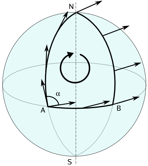
The Riemann tensor precisely quantifies this phenomenon for an infinitesimally small loop. It measures the failure of a vector to return to itself after being parallel transported around an infinitesimal parallelogram.

To get a feel for this geometric idea, the following video provides an excellent introduction.

2. The Formal Definition: Commutator of Covariant Derivatives

The mathematical counterpart to the path-dependence of parallel transport is the fact that covariant derivatives do not, in general, commute. In flat space with Cartesian coordinates, second partial derivatives commute: ${\partial }_{\mu }{\partial }_{\nu }f={\partial }_{\nu }{\partial }_{\mu }f$. In curved space, the order of covariant differentiation matters, and the difference between ${\nabla }_{\mu }{\nabla }_{\nu }$ and ${\nabla }_{\nu }{\nabla }_{\mu }$ is precisely the measure of curvature.

Let's compute the action of the commutator of two covariant derivatives, $[{\nabla }_{\mu },{\nabla }_{\nu }]={\nabla }_{\mu }{\nabla }_{\nu }-{\nabla }_{\nu }{\nabla }_{\mu }$, on a vector field $V^{\rho }$. This calculation is the cornerstone of this lesson.

You will now study the rigorous derivation from one of two excellent sources. Both arrive at the same fundamental result. You can choose the one whose style you prefer.

Alternatively, David Tong's notes offer a slightly more expansive but equally rigorous derivation.

Both derivations show that for a general connection, the commutator acting on a vector is given by the Ricci Identity:

where $T^{\lambda }{}_{\mu \nu }={\Gamma }_{\mu \nu }^{\lambda }-{\Gamma }_{\nu \mu }^{\lambda }$ is the torsion tensor.

Since we are working with the unique metric-compatible, torsion-free Levi-Civita connection, we have $T^{\lambda }{}_{\mu \nu }=0$. The Ricci Identity simplifies to:

This equation serves as the definition of the Riemann curvature tensor. It states that the Riemann tensor is the linear operator that maps a vector $V^{\sigma }$ to the "error" vector generated by swapping the order of two covariant derivatives.

The components of this (1, 3) tensor are given by the expression derived in the readings:

Notice that the Riemann tensor is constructed entirely from the connection coefficients and their first derivatives. If we can find a coordinate system where the metric is constant everywhere, the connection coefficients vanish, and thus $R^{\rho }{}_{\sigma \mu \nu }=0$. Since this is a tensor equation, if it is zero in one coordinate system, it is zero in all. A vanishing Riemann tensor is the true hallmark of a flat spacetime.

3. The Coordinate-Free Definition

While the component form is essential for calculations, a more profound and coordinate-independent definition exists. The Riemann tensor $R$ can be defined as a map that takes three vector fields $X,Y,Z$ and returns a fourth vector field $R(X,Y)Z$.

For any three vector fields $X,Y,Z$, the Riemann curvature tensor is defined as:

Here, ${\nabla }_X$ is the covariant derivative along the vector field $X$, and $[X,Y]$ is the Lie bracket of $X$ and $Y$, which we have encountered previously.

Why the extra term?
The term $-{\nabla }_{[X,Y]}Z$ is crucial. It ensures that $R(X,Y)Z$ is a true tensor—meaning it is linear over functions in its arguments $X,Y$, and $Z$. Without this term, the expression would not be a tensor. Your mathematical background makes you well-placed to appreciate this point of rigor.

If you choose your vector fields $X$ and $Y$ to be coordinate basis vectors, $X={\partial }_{\mu }$ and $Y={\partial }_{\nu }$, their Lie bracket vanishes, i.e., $[{\partial }_{\mu },{\partial }_{\nu }]=0$. In this case, the definition simplifies to:

This connects the elegant coordinate-free definition to the component formula we derived earlier.

4. Physical Interpretation Revisited: Geodesic Deviation

The commutator of derivatives can feel abstract. Let's connect our new tensor to another powerful physical idea: tidal forces.

In a uniform gravitational field, two nearby falling objects would remain perfectly parallel. In a non-uniform field, like Earth's, they will accelerate relative to one another. Two objects dropped side-by-side will accelerate towards each other as they fall towards the Earth's center. This relative acceleration is a tidal effect.

In General Relativity, this phenomenon is called geodesic deviation. The worldlines of two nearby freely-falling particles are geodesics. In a curved spacetime, these geodesics will in general accelerate towards or away from each other. The Riemann tensor governs this relative acceleration.

If $U^{\mu }$ is the four-velocity tangent to a family of geodesics and $S^{\mu }$ is the vector connecting two nearby geodesics, their relative acceleration is given by the geodesic deviation equation:

where $\frac{D}{d\tau }=U^{\nu }{\nabla }_{\nu }$ is the covariant derivative along the worldline.

This equation provides a direct physical interpretation of the Riemann tensor: it is the object that determines the tidal forces of gravity. If the Riemann tensor is zero, there is no geodesic deviation, and initially parallel free-fall paths remain parallel, just as in flat spacetime.

Conclusion

In this lesson, we have formally defined the central object for describing spacetime curvature.

Key Takeaways:

• The Christoffel symbols are not tensors and cannot be used as a measure of intrinsic curvature.
• Intrinsic curvature manifests physically as the path-dependence of parallel transport (holonomy) and as tidal forces (geodesic deviation).
• The Riemann curvature tensor is the mathematical object that quantifies curvature. It is zero if and only if a spacetime is flat.
• It is fundamentally defined by the failure of covariant derivatives to commute. For a torsion-free connection, this relationship is $({\nabla }_{\mu }{\nabla }_{\nu }-{\nabla }_{\nu }{\nabla }_{\mu })V^{\rho }=R^{\rho }{}_{\sigma \mu \nu }{V}^{\sigma }$.
• Its components are constructed from the connection coefficients and their first derivatives: $R^{\rho }{}_{\sigma \mu \nu }={\partial }_{\mu }{\Gamma }_{\nu \sigma }^{\rho }-{\partial }_{\nu }{\Gamma }_{\mu \sigma }^{\rho }+{\Gamma }_{\mu \lambda }^{\rho }{\Gamma }_{\nu \sigma }^{\lambda }-{\Gamma }_{\nu \lambda }^{\rho }{\Gamma }_{\mu \sigma }^{\lambda }$.

We have now defined the Riemann tensor. However, in four dimensions, it naively has $4^4=256$ components! This is a terrifyingly large number. Fortunately, the tensor possesses a rich set of algebraic symmetries that drastically reduce the number of independent components.

In our next lesson, we will explore these crucial algebraic symmetries of the Riemann tensor and the Bianchi identities. This will be our next step towards understanding the structure of curved spacetime and, ultimately, formulating the Einstein Field Equations.