Levi-Civita Connection: From Metric Compatibility to Torsion-Free

Hello! Welcome back to our course.

In our last lesson, we introduced the affine connection, $\nabla$ , as the essential tool for differentiating tensor fields on a manifold. We saw that the ordinary partial derivative fails because it isn't a coordinate-independent operation. The connection, represented in coordinates by the coefficients $Γ_{μν}^{λ}$ , provides the necessary "correction" to define a true tensor operator—the covariant derivative.

However, we left a crucial question unanswered: on a given manifold, there can be infinitely many possible connections. Which one should we use? Today's lesson will provide the answer for the spacetimes of General Relativity. We will show that if a manifold is endowed with a metric tensor $g_{μν}$ , a unique and physically natural connection is singled out.

This lesson's learning outcome is to derive the Levi-Civita connection from the metric compatibility and torsion-free conditions. This derivation is a cornerstone of Riemannian geometry and, by extension, General Relativity, as it establishes the fundamental link between the metric (which will play the role of the gravitational potential) and the notion of differentiation and curvature.

1. Two Conditions for a Unique Connection

In physics, and particularly in GR, we want a connection that respects the geometric structure already present on the manifold. The most important structure we have is the metric tensor, $g_{μν}$ , which defines lengths and angles. We will impose two reasonable conditions on our connection that tie it to the metric. These conditions will prove to be so restrictive that they determine the connection uniquely.

Condition 1: Metric Compatibility

The first and most important condition is that the connection must be compatible with the metric. This means that the metric tensor is constant under covariant differentiation. Formally, we require:

\nabla_{σ} g_{μν} = 0

This is called the metric compatibility condition.

What does this mean intuitively? In the last lesson, we hinted that the connection defines parallel transport—a way to move vectors along curves while keeping them "pointing in the same direction". Metric compatibility ensures that this process preserves the metric structure. Specifically, if you parallel-transport two vectors $V$ and $U$ along a curve, their inner product $g (V, U)$ will remain constant. Consequently, the lengths of vectors and the angles between them are preserved during parallel transport.

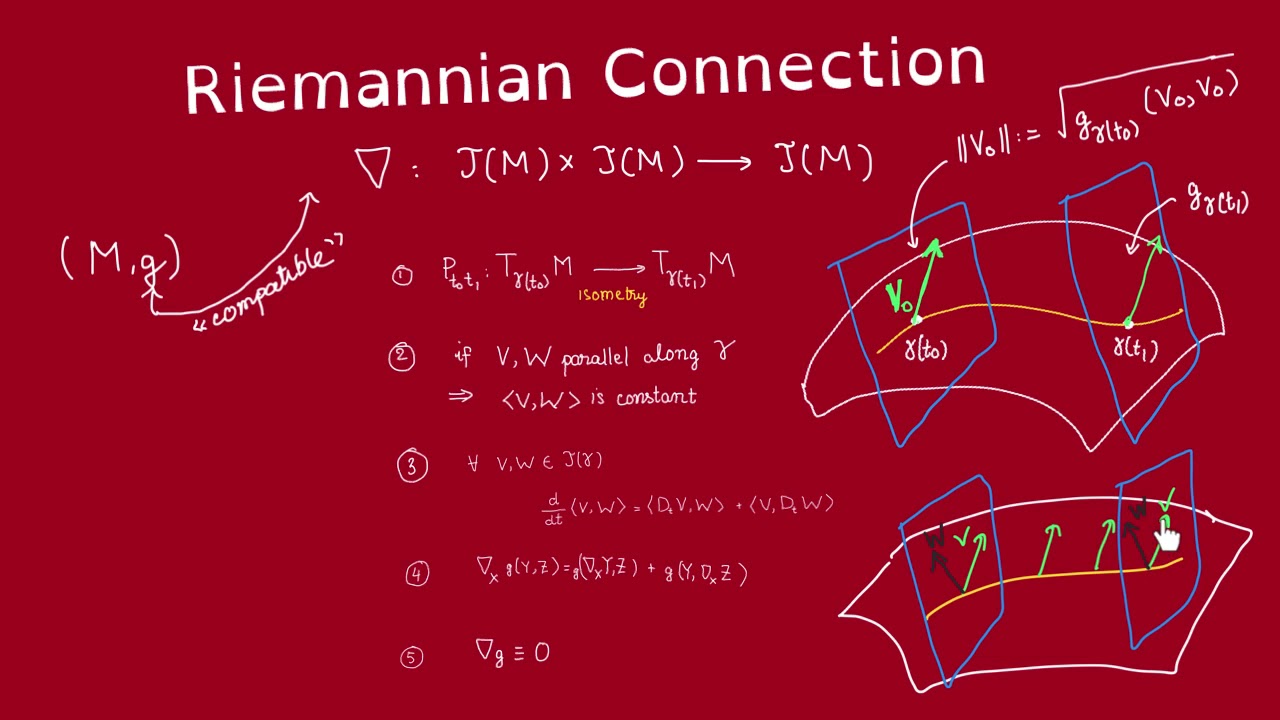
Riemannian Connection Properties and Visualization — This image illustrates the core idea of metric compatibility. As vectors are parallel transported along a curve on the manifold, their lengths and the angle between them (determined by the metric $g$) remain unchanged. This is a direct consequence of the condition $\nabla g = 0$.

A powerful practical consequence of metric compatibility is that the covariant derivative commutes with raising and lowering indices. For example, for a vector field $V^{μ}$ , its one-form counterpart is $V_{ν} = g_{ν μ} V^{μ}$ . Then:

\nabla_{σ} V_{ν} = \nabla_{σ} (g_{ν μ} V^{μ}) = (\nabla_{σ} g_{ν μ}) V^{μ} + g_{ν μ} (\nabla_{σ} V^{μ})

Since $\nabla_{σ} g_{ν μ} = 0$ , we simply get:

\nabla_{σ} V_{ν} = g_{ν μ} (\nabla_{σ} V^{μ})

This simplifies calculations immensely.

Condition 2: Torsion-Free

The second condition we impose is that the connection is torsion-free, or symmetric. Algebraically, this means the connection coefficients are symmetric in their lower two indices:

Γ_{μν}^{λ} = Γ_{ν μ}^{λ}

This condition is equivalent to the vanishing of the torsion tensor, which is defined as $T_{μν}^{λ} = Γ_{μν}^{λ} - Γ_{ν μ}^{λ}$ .

The geometric meaning of zero torsion is that infinitesimal parallelograms close. If you move an infinitesimal distance along a vector $X$ and then along a vector $Y$ , you arrive at the same point as if you had moved first along $Y$ and then along $X$ . In terms of covariant derivatives, the torsion-free condition is equivalent to the statement:

\nabla_{X} Y - \nabla_{Y} X = [X, Y]

where $[X, Y]$ is the Lie bracket of the vector fields, which you'll recall from our first module. In a coordinate basis where $[\partial_{μ}, \partial_{ν}] = 0$ , this directly implies the symmetry of the connection coefficients. While theories of gravity with torsion exist (like Einstein-Cartan theory), General Relativity is built upon a torsion-free connection.

Now, let's watch a short video that introduces these two defining properties before we use them in our derivation.

Tensor Calculus 20: The Abstract Covariant Derivative (Levi-Civita Connection)

The YouTuber eigenchris provides a clear explanation of both the torsion-free and metric compatibility properties. This will help solidify your intuition for what these conditions mean before we dive into the algebra.

Please watch from 10:24 to 14:20. 10:24 - 12:00: Focus on the definition of the torsion-free property and how it implies the symmetry of Christoffel symbols. 12:00 - 14:20: Pay close attention to the explanation of metric compatibility. The video gives the excellent physical interpretation that dot products (and thus lengths and angles) are preserved under parallel transport.

2. Deriving the Levi-Civita Connection

We now have our two conditions:

Metric Compatibility: $\nabla_{σ} g_{μν} = 0$
Torsion-Free: $Γ_{μν}^{λ} = Γ_{ν μ}^{λ}$

Our goal is to use these to find a unique formula for $Γ_{μν}^{λ}$ in terms of the metric $g_{μν}$ and its derivatives. This will prove both the existence and uniqueness of such a connection.

Let's start by writing out the metric compatibility condition using the general formula for the covariant derivative of a (0,2) tensor:

\nabla_{σ} g_{μν} = \partial_{σ} g_{μν} - Γ_{μ σ}^{λ} g_{λ ν} - Γ_{ν σ}^{λ} g_{μ λ} = 0

This can be rearranged into our starting equation:

\partial_{σ} g_{μν} = Γ_{μ σ}^{λ} g_{λ ν} + Γ_{ν σ}^{λ} g_{μ λ}

This equation contains the unknown $Γ$ s we want to solve for. The trick is to write this equation three times with cyclically permuted indices, and then add and subtract them in a clever way.

Let's write down the three equations:

$\partial_{σ} g_{μν} = Γ_{μ σ}^{λ} g_{λ ν} + Γ_{ν σ}^{λ} g_{μ λ}$
$\partial_{μ} g_{ν σ} = Γ_{ν μ}^{λ} g_{λσ} + Γ_{σ μ}^{λ} g_{ν λ}$
$\partial_{ν} g_{σ μ} = Γ_{σ ν}^{λ} g_{λ μ} + Γ_{μν}^{λ} g_{σ λ}$

Now, we compute the combination (2) + (3) - (1). The left-hand side is simply $\partial_{μ} g_{ν σ} + \partial_{ν} g_{σ μ} - \partial_{σ} g_{μν}$ . Let's examine the right-hand side:

(Γ_{ν μ}^{λ} g_{λσ} + Γ_{σ μ}^{λ} g_{ν λ}) + (Γ_{σ ν}^{λ} g_{λ μ} + Γ_{μν}^{λ} g_{σ λ}) - (Γ_{μ σ}^{λ} g_{λ ν} + Γ_{ν σ}^{λ} g_{μ λ})

This looks complicated, but now we apply our two simplifying conditions:

Torsion-free: $Γ_{μν}^{λ} = Γ_{ν μ}^{λ}$ , etc.
Metric symmetry: $g_{μν} = g_{ν μ}$

Let's look for cancellations:

The term $Γ_{σ μ}^{λ} g_{ν λ}$ from (2) cancels with $- Γ_{μ σ}^{λ} g_{λ ν}$ from (1), because $Γ_{σ μ}^{λ} = Γ_{μ σ}^{λ}$ and we can relabel the dummy indices $λ \leftrightarrow ν$ in one term. More directly, look at the terms: $+ Γ_{σ μ}^{λ} g_{ν λ}$ and $- Γ_{μ σ}^{λ} g_{λ ν}$ . Using torsion-free, the first is $Γ_{μ σ}^{λ} g_{ν λ}$ . Using metric symmetry, the second is $- Γ_{μ σ}^{λ} g_{ν λ}$ . They cancel.
Similarly, $Γ_{σ ν}^{λ} g_{λ μ}$ from (3) cancels with $- Γ_{ν σ}^{λ} g_{μ λ}$ from (1).

After these cancellations, only two terms remain on the right-hand side:

Γ_{ν μ}^{λ} g_{λσ} + Γ_{μν}^{λ} g_{σ λ}

Using the torsion-free condition again ( $Γ_{ν μ}^{λ} = Γ_{μν}^{λ}$ ) and the metric symmetry ( $g_{σ λ} = g_{λσ}$ ), these two terms are identical. So the right-hand side simplifies to $2 Γ_{μν}^{λ} g_{λσ}$ .

Putting it all together, we have:

\partial_{μ} g_{ν σ} + \partial_{ν} g_{σ μ} - \partial_{σ} g_{μν} = 2 Γ_{μν}^{λ} g_{λσ}

We are almost there! To isolate $Γ$ , we multiply both sides by the inverse metric $g^{σ ρ}$ :

\frac{1}{2} g^{σ ρ} (\partial_{μ} g_{ν σ} + \partial_{ν} g_{σ μ} - \partial_{σ} g_{μν}) = g^{σ ρ} Γ_{μν}^{λ} g_{λσ} = δ_{λ}^{ρ} Γ_{μν}^{λ} = Γ_{μν}^{ρ}

Relabeling the free index $ρ$ to $λ$ for convention, we arrive at the final result:

Γ_{μν}^{λ} = \frac{1}{2} g^{λσ} (\partial_{μ} g_{ν σ} + \partial_{ν} g_{μ σ} - \partial_{σ} g_{μν})

This celebrated formula explicitly gives the connection coefficients in terms of the metric and its first partial derivatives. This unique, torsion-free, metric-compatible connection is called the Levi-Civita connection (or sometimes the Riemannian or Christoffel connection). The coefficients $Γ_{μν}^{λ}$ are often called the Christoffel symbols of the second kind.

The following resources provide a complete walkthrough of this essential derivation.

Lecture Notes on General Relativity - S. Carroll

Sean Carroll's lecture notes provide a clear and concise derivation that is standard in many GR textbooks. It follows the exact logic we just used.

Please read the last two subsections of Section 3 of the notes. Start at the text introducing the 'torsion-free' and 'metric compatibility' properties. This will formalize the two conditions. Then, carefully follow the derivation from equation (3.19) to the final result in equation (3.21). This is the algebraic heart of today's lesson.

Tensor Calculus 20: The Abstract Covariant Derivative (Levi-Civita Connection)

For a video walkthrough, eigenchris again provides an excellent presentation of the same derivation, which can help clarify any steps that seem dense in the text.

Watch the segment from 14:20 to 16:53. This part of the video explicitly carries out the cyclic permutation and algebraic manipulation to arrive at the final formula for the Christoffel symbols, just as we did above.

This result is called the Fundamental Theorem of Riemannian Geometry. It states that on any Riemannian (or pseudo-Riemannian) manifold, there exists a unique connection that is both metric-compatible and torsion-free.

Test your understanding!

Imagine a 2D Euclidean plane described by polar coordinates $(r, \theta)$. The metric is given by $ds^2 = dr^2 + r^2 d\theta^2$. This means the only non-zero metric components are $g_{rr}=1$ and $g_{\theta\theta}=r^2$. The inverse metric components are $g^{rr}=1$ and $g^{\theta\theta}=1/r^2$.

Using the Levi-Civita formula, calculate the Christoffel symbol $Γ_{θ θ}^{r}$ .

Show answer

We want to calculate $Γ_{θ θ}^{r}$ . In the formula, this corresponds to $λ = r$ , $μ = θ$ , $ν = θ$ .
The formula is:
$Γ_{μν}^{λ} = \frac{1}{2} g^{λσ} (\partial_{μ} g_{ν σ} + \partial_{ν} g_{μ σ} - \partial_{σ} g_{μν})$
Let's plug in our indices:
$Γ_{θ θ}^{r} = \frac{1}{2} g^{r σ} (\partial_{θ} g_{θ σ} + \partial_{θ} g_{θ σ} - \partial_{σ} g_{θ θ}) = \frac{1}{2} g^{r σ} (2 \partial_{θ} g_{θ σ} - \partial_{σ} g_{θ θ})$
The summation is over $σ$ , which can be $r$ or $θ$ . Also, $g^{r σ}$ is only non-zero for $σ = r$ (where $g^{r r} = 1$ ). So we only need to consider the $σ = r$ term in the sum:
$Γ_{θ θ}^{r} = \frac{1}{2} g^{r r} (2 \partial_{θ} g_{θ r} - \partial_{r} g_{θ θ})$
Now we evaluate the terms:

$g^{r r} = 1$
$g_{θ r} = 0$ , so $\partial_{θ} g_{θ r} = 0$ .
$g_{θ θ} = r^{2}$ , so $\partial_{r} g_{θ θ} = \partial_{r} (r^{2}) = 2 r$ .

Plugging these values in:
$Γ_{θ θ}^{r} = \frac{1}{2} (1) (2 (0) - 2 r) = \frac{1}{2} (- 2 r) = - r$
So, $Γ_{θ θ}^{r} = - r$ . This non-zero Christoffel symbol is a manifestation of the fact that polar coordinates are a curvilinear system on a flat space; the basis vectors $r^$ and $θ^$ change direction from point to point.

Conclusion

This lesson has been pivotal. We have closed the conceptual gap from the previous lesson and established the unique connection that underpins General Relativity.

Key Takeaways:

On a manifold with a metric, we can single out a unique connection by imposing two conditions: metric compatibility ( $\nabla g = 0$ ) and zero torsion ( $Γ_{μν}^{λ} = Γ_{ν μ}^{λ}$ ).
Metric compatibility means that inner products, lengths, and angles are preserved under parallel transport.
Zero torsion means that the connection is symmetric in its lower indices, which corresponds to infinitesimal parallelograms closing.
These two conditions lead to a unique solution for the connection coefficients, known as the Christoffel symbols, in terms of the metric and its first derivatives.
This unique connection is called the Levi-Civita connection, and its existence and uniqueness constitute the Fundamental Theorem of Riemannian Geometry.

We now have a complete, unambiguous toolkit for differentiation on a (pseudo-)Riemannian manifold. The metric determines the connection, and the connection tells us how to differentiate tensors.

In our next lesson, we will make the concept of "moving a vector along a curve while keeping it constant" precise by formally defining parallel transport. This will immediately lead us to one of the most important equations in physics: the geodesic equation, which describes the paths of freely falling particles in curved spacetime.

Recommended resources

1. Two Conditions for a Unique Connection

Condition 1: Metric Compatibility

Condition 2: Torsion-Free

2. Deriving the Levi-Civita Connection

Conclusion