Welcome to our second-to-last lesson in the course.
In our previous session, we reached the top of Pearl's Ladder of Causation by exploring counterfactuals. We learned that to answer "what if" questions, a causal graph is not enough; we need a full Structural Causal Model (SCM) that specifies the underlying mechanisms. We walked through the three-step algorithm—Abduction, Action, Prediction—for computing counterfactuals, assuming the SCM was known and correct.
This naturally leads to a fundamental epistemological question: How do we determine the correct causal model in the first place? In the real world, we rarely have a pre-verified SCM. Instead, we have data and competing causal hypotheses. For instance, in your field of social research, does a couple's communication style influence their relationship satisfaction, or does their baseline satisfaction level drive their communication style? Or is there a third factor, like shared values, that influences both?
Today's lesson addresses this challenge directly, fulfilling the learning outcome: Describe how Bayesian methods can be used to update beliefs about the structure of a causal model in light of new evidence. We will see how the principles of Bayesian epistemology provide a formal and powerful engine for learning about causal structure from data, allowing us to quantify and systematically revise our beliefs about how the world works.
1. Causal Inference as a Bayesian Problem
The bridge between causality and Bayesianism is the shared challenge of reasoning under uncertainty. In causal inference, this uncertainty can exist at multiple levels: uncertainty about the value of a parameter, uncertainty about a counterfactual outcome, or, most fundamentally, uncertainty about the causal structure itself.
A powerful framing, pioneered by Donald Rubin, is to view causal inference as a missing data problem. When we observe a person who took a drug and recovered, the counterfactual outcome—what would have happened had they not taken the drug—is a piece of missing data. The Bayesian approach provides a unified framework for handling such problems.
Tutorial | Bayesian causal inference: A critical review and tutorial (Standard Format)
To start, let's watch a segment of a tutorial from the Harvard Data Science Initiative that introduces this perspective.
Watch from 09:29 to 12:04. The speaker explains how causal inference can be viewed as a structured missing data problem and how this insight connects the work of Donald Rubin on both topics. The key idea is that we can use Bayesian inference to impute these missing values by treating them as unobserved random variables.
The core of the Bayesian method is to define a joint probability distribution over all quantities of interest—both observed and unobserved. This includes the data, model parameters, and, as we'll see, the very structure of the model.
Tutorial | Bayesian causal inference: A critical review and tutorial (Standard Format)
This next segment from the same video lays out the formal Bayesian setup. While it's presented in the context of estimating causal effects, the principle is general.
Watch from 21:25 to 26:23. Pay close attention to the slide that decomposes the full joint distribution into three parts: the assignment mechanism, the outcome model, and the covariate distribution. As a statistician, you'll recognize this factorization. The philosophical point is that by specifying a complete probabilistic model of the world, we can then use the machinery of Bayesian inference to learn about any part of it from evidence.
This sets the stage for our main topic. If we can use Bayesian methods to learn about unknown parameters or unobserved outcomes within a given model, can we use the same logic to learn about the model itself? The answer is yes.
2. Bayesian Networks and Belief Updating
Before tackling structure learning, let's quickly review how a Bayesian Network (BN) works. A BN is a Directed Acyclic Graph (DAG) where each node represents a random variable and the arrows represent probabilistic dependencies. Each node is equipped with a probability table that specifies its probability conditional on its parents. A BN is a compact representation of a joint probability distribution.
The power of a BN is that it's not just a static representation; it's an engine for reasoning. When we observe the value of a variable (i.e., we get evidence), we can propagate that information through the network to update our beliefs about all other variables. This is a direct application of Bayes' rule.
The following short video provides a simple, clear demonstration of this process.
Watch the video from the beginning to 03:02. Notice how observing evidence—like 'patient is a non-smoker' or 'x-ray is positive'—changes the probabilities of the diagnoses ('lung cancer', 'tuberculosis'). This is belief updating in action on a graphical model.
When we stipulate that the arrows in a BN represent causal relationships, it becomes a Causal Bayes Net, inheriting the properties we've discussed for SCMs. Today, our goal is to use this updating mechanism not just to update beliefs about the state of variables within a graph, but to update our beliefs about the graph itself.
3. Bayesian Causal Structure Learning
We can frame the problem of learning a causal structure as a form of Bayesian model selection. Here’s how the components map:
- Hypothesis Space (): The set of all possible causal graphs we are considering. For two variables and , the hypotheses might be , , or no edge between them.
- Priors (): Our initial degree of belief in each causal structure before seeing the data. We might start with a uniform prior (all graphs are equally likely) or use prior knowledge to favor certain structures.
- Likelihood (): The probability of observing our data if graph were the true causal structure of the world.
- Posterior (): Our updated degree of belief in each causal graph after observing the data.
The posterior is calculated using Bayes' rule, just as we've seen throughout this course:
This approach transforms the ambiguous task of "discovering causes" into a formal problem of probabilistic inference.
The following resource provides a detailed, real-world example of this process, along with the technical implementation of the Bayesian analysis.
Causal Imprinting in Causal Structure Learning
Let's read a few sections from a fascinating paper titled 'Causal Imprinting in Causal Structure Learning'. The paper investigates a scenario where an initial belief (B causes C) is challenged by new evidence suggesting a common cause (A causes both B and C). The authors use a Bayesian model as a normative standard to analyze how a rational agent should update their belief about the causal structure.
Please read sections 3.1 ('Preview of Bayesian analyses'), 3.2 ('Modeling methods'), and 3.3 ('Modeling results'). Section 3.1 gives a conceptual overview. Section 3.2 details the application of Bayes' rule (Equation 1) and the method for calculating the likelihood of the data given a hypothesis (Equations 2-4). Section 3.3 shows the results: the posterior probabilities for each of the eight possible causal structures (Table 1). This is a concrete demonstration of the lesson's learning outcome.
The methods described in the paper show precisely how to translate a philosophical principle—updating beliefs in light of evidence—into a concrete computational procedure for learning causal graphs.
4. The Cycle of Discovery and Its Epistemological Wrinkles
The Bayesian learning process is not a one-time calculation. It is a dynamic, iterative cycle at the heart of scientific discovery.
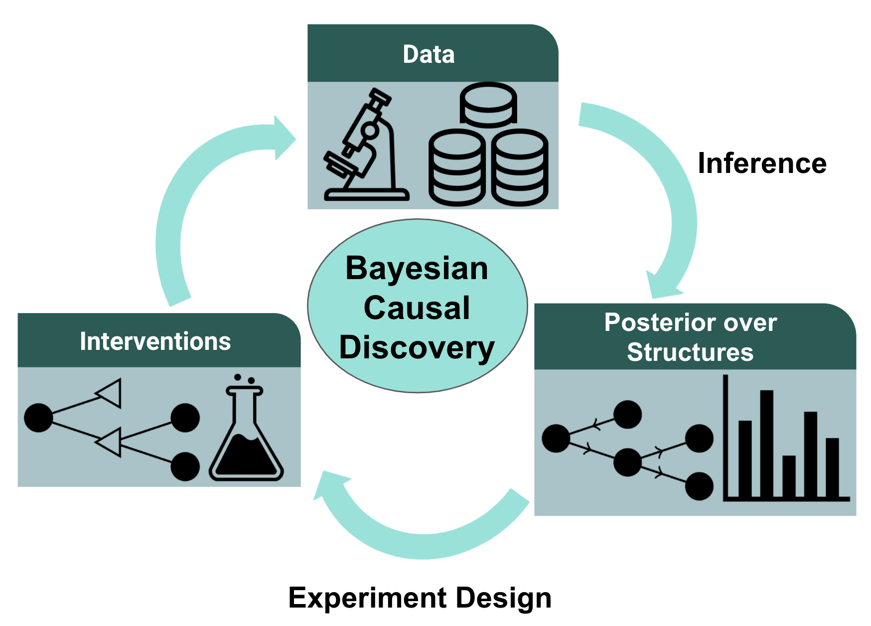
This cycle represents a formal model of scientific epistemology: we update our theories (causal graphs) with data, and our updated theories guide our future search for evidence.
However, the "Causal Imprinting" paper you just read reveals a critical wrinkle. The Bayesian model provides a normative standard for how a perfectly rational agent should update their beliefs. But do humans, even scientists, reason this way?
The paper's main finding is that people exhibit "causal imprinting": they tend to stick with their initial causal belief (e.g., ) even after seeing evidence of a common cause that normatively should make them discard it. Their final belief state is different from the posterior distribution calculated by the Bayesian model. This highlights a key theme of our course: the distinction between Bayesianism as a normative theory of rationality and a descriptive theory of human cognition.
Conclusion
Today, we have connected the two major threads of this course: causal modeling and Bayesian epistemology. We've seen that Bayesian inference isn't just for updating beliefs about parameters within a model; it's a powerful framework for learning the structure of the model itself.
Key Takeaways:
- Structure Learning as Bayesian Inference: The problem of discovering causal structure can be formalized as a Bayesian model selection problem, where we calculate the posterior probability of different causal graphs given data.
- The Machinery: The process involves defining a hypothesis space of graphs, assigning priors, calculating the likelihood of data under each graph, and using Bayes' rule to find the posterior distribution over graphs.
- A Unified Framework: The Bayesian approach provides a coherent way to reason under uncertainty, whether it's about missing data, counterfactual outcomes, or the causal structure of the world.
- Normative vs. Descriptive: While Bayesian structure learning provides a normative standard for rational belief revision, human reasoning can sometimes deviate, as shown by phenomena like "causal imprinting."
- The Cycle of Discovery: This process forms an iterative loop of inference and experimentation, formalizing a key aspect of scientific discovery.
In our final lesson, we will synthesize everything we've learned. We will take a single case study—a variant of Simpson's Paradox—and analyze it from start to finish, demonstrating how causal and Bayesian reasoning combine to untangle complexity and guide decision-making.