Solving First-Order Linear Equations with Initial Conditions

From General to Particular Solutions

A general solution, like $y(x)=\sin (x)+C\cos (x)$ from our last lesson, describes a whole family of solution curves. Each value of $C$ gives a different curve.

An initial condition is a specified point, $(x_0,y_0)$, that the solution curve must pass through. By forcing our general solution to pass through this point, we can determine the exact value of $C$. The resulting function, with a specific numerical value for $C$, is called the particular solution.

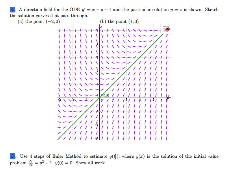
Visually, think of a direction field, which shows the slope of the solution at every point. The general solution represents all possible paths you could draw that follow these slopes. An initial condition is like placing your pencil at a starting point; there's only one path you can trace from there.

The Process for Solving an Initial Value Problem

The process is a straightforward extension of what we've already learned. It adds one final algebraic step.

As you saw, the strategy is:

1. Put the equation into standard form: $y^{\prime }+p(x)y=q(x)$.
2. Calculate the integrating factor: $\mu (x)=e^{\int p(x)dx}$.
3. Multiply the equation by $\mu (x)$ and recognize the left side as $\frac{d}{dx}[\mu (x)y]$.
4. Integrate both sides to find the general solution for $y(x)$.
5. Apply the initial condition: Substitute the given values of $x_0$ and $y_0$ into the general solution and solve for the constant $C$. This gives you the particular solution.

Applying the Final Step: A Familiar Example

Let's revisit the last example from our previous lesson:
$\cos (x)y^{\prime }+\sin (x)y=1$
We found the general solution to be:
$y(x)=\sin (x)+C\cos (x)$
Now, let's turn this into an Initial Value Problem by adding the initial condition $y(\pi )=2$. This means when $x=\pi$, $y$ must be 2.

Step 5: Find C
We substitute $x=\pi$ and $y=2$ into our general solution:
$2=\sin (\pi )+C\cos (\pi )$
We know that $\sin (\pi )=0$ and $\cos (\pi )=-1$.
$2=0+C(-1)$
$2=-C$
$C=-2$
Now we substitute this value of $C$ back into the general solution to get our particular solution:
$y(x)=\sin (x)-2\cos (x)$
This is the unique function that both satisfies the differential equation and passes through the point $(\pi ,2)$.

The following short video clip demonstrates this exact process for the problem we just solved.

Practice: Solving IVPs from Start to Finish

Now let's work through some complete examples. The following video resource presents two Initial Value Problems and solves them using the five-step method. For each one, I'll ask you to watch the corresponding section.

Example 1: A Standard IVP
Solve the IVP: $\frac{dy}{dx}+2y=e^{2x}$, with the initial condition $y(0)=3$.

This problem is already in standard form, so we can proceed directly. Please watch the solution to this first example.

Example 2: An IVP Requiring Standard Form
Solve the IVP: $x{y}^{\prime }+y=x$, with the initial condition $y(2)=4$.

Here, you must first put the equation into standard form before finding the integrating factor.

These examples reinforce the entire process, from setting up the equation to finding the final particular solution.

Conclusion

Congratulations on completing the first module! We have built a complete and reliable method for solving any first-order linear differential equation, including those with initial conditions.

Key Takeaways:

• A general solution contains the constant $C$ and represents a family of functions.
• An Initial Value Problem (IVP) consists of a differential equation and an initial condition, like $y(x_0)=y_0$.
• The initial condition allows us to solve for $C$ and find a unique particular solution.
• The process is to first find the general solution using the integrating factor method, then substitute the initial condition to determine the value of $C$.

Preview of the next lesson:
We now have a solid foundation in first-order equations. In our next lesson, we will move up an order of complexity and begin Module 2: Second-Order Homogeneous Equations. We will start by learning how to formulate and solve the "characteristic equation," which is the key to solving a large class of second-order differential equations.