NFA-ε: Definition and Conversion to NFA

Why Add ε-Transitions?

So far, our automata could only change state after reading an input symbol. An NFA-ε introduces a new capability: the ability to change state without consuming any input. This is represented by an ε-transition, sometimes called a "null" or "empty" transition.

Why is this useful? Think about the regular expression a*. It represents zero or more a's. An ε-transition provides a natural way to model the "zero" case or the optionality inherent in the Kleene star and union operators. These "free moves" make it much easier to build automata directly from regular expressions, as we'll see in our next lesson.

Formal Definition of an NFA-ε

An NFA-ε is very similar to a standard NFA, with one key change to the transition function.

As the video explains, an NFA-ε is a 5-tuple $M=(Q,\Sigma ,\delta ,q_0,F)$, where:

• $Q$ is the finite set of states.
• $\Sigma$ is the input alphabet.
• $\delta$ is the transition function, $\delta :Q\times (\Sigma \cup \{ϵ\})\to \mathcal{P}(Q)$. This is the crucial difference: the function now accepts the empty string $ϵ$ as a possible input.
• $q_0$ is the start state.
• $F$ is the set of final states.

The power of an NFA-ε comes from its ability to be in multiple states at once, not just through nondeterministic choices on an input symbol, but also by following these "free" ε-paths simultaneously.

The ε-Closure: Tracking All Possible "Free" Moves

To work with an NFA-ε, we need a way to track all the states the machine could possibly be in at any given moment, including all the states reachable through ε-jumps. This is the job of the ε-closure.

The ε-closure of a state $q$, written as ε-closure(q) or E(q), is the set of all states reachable from $q$ by following zero or more ε-transitions.

• Zero ε-moves: A state is always in its own ε-closure.
• One or more ε-moves: We follow all possible paths of ε-transitions from $q$ and add every state we visit to the set.

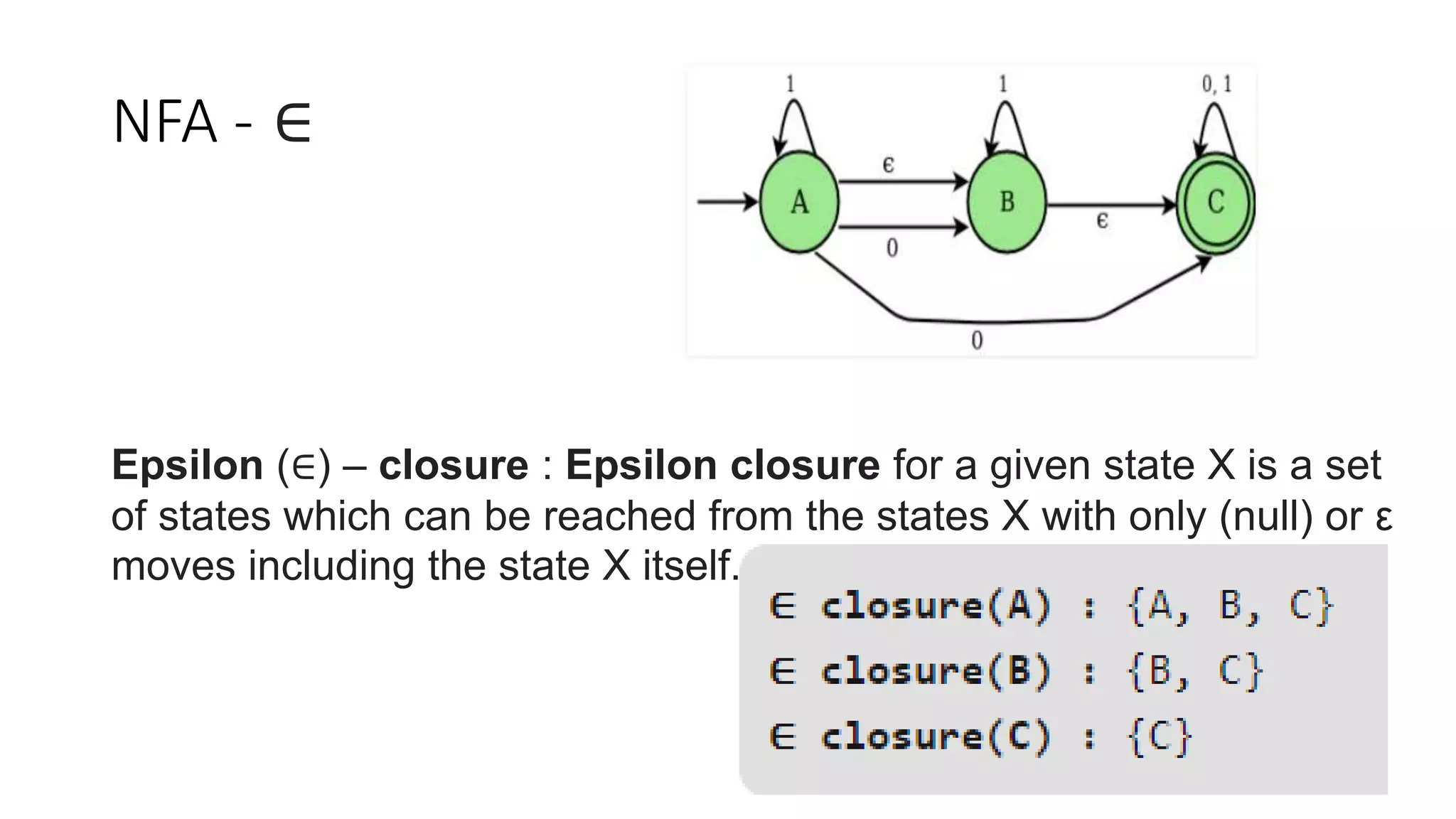
The following video provides a more formal definition and a clear, animated example of how to compute the ε-closure.

Converting an NFA-ε to an Equivalent NFA

Our next step is to prove that ε-transitions, while convenient, do not add any fundamental power to our machines. We do this by showing that for any NFA-ε $N$, we can construct a standard NFA $N^{\prime }$ that accepts the same language.

The Core Idea: A single transition in our new NFA $N^{\prime }$ on an input symbol a will simulate a three-step process in the original NFA-ε $N$:

1. First, make any possible ε-moves.
2. Then, consume the single input symbol a.
3. Finally, make any subsequent ε-moves.

This logic is captured formally in the definition of the new transition function, ${\delta }^{\prime }$.

Let's break down that crucial formula: ${\delta }^{\prime }(q,a)=\text{ε-closure}(\delta (\text{ε-closure}(q),a))$

1. ε-closure(q): This is Step 1. Start at state $q$ and find all states reachable via free ε-moves. Let's call this set of states $S$.
2. δ(S, a): This is Step 2. From all the states in $S$, find where you can go by consuming the single input symbol $a$. Let this new set of states be $T$.
3. ε-closure(T): This is Step 3. From all the states in $T$, find all the states you can now reach via another set of free ε-moves. This final set is the result for ${\delta }^{\prime }(q,a)$.

The construction of the equivalent NFA $N^{\prime }=(Q,\Sigma ,{\delta }^{\prime },q_0,F^{\prime })$ is as follows:

• States: The states are the same, $Q$.
• Alphabet: The alphabet is the same, $\Sigma$.
• Start State: The start state is the same, $q_0$.
• Transition Function: ${\delta }^{\prime }$ is computed using the formula above for every state and every symbol in $\Sigma$.
• Final States ($F^{\prime }$): This is the last piece. A state $q$ in $N^{\prime }$ is a final state if its ε-closure in $N$ (the original machine) contains at least one of the original final states from $F$. Formally, $F^{\prime }=\{q\in Q\mid \text{ε-closure}(q)\cap F\ne \varnothing \}$.

The image below gives a complete visual walkthrough of this process, from the original NFA-ε to the final NFA transition table.

An Alternative View: Edge Duplication

For those who prefer a more graphical approach, you can also think of the conversion as "bypassing" the ε-transitions. If you have a path p --ε--> q --a--> r, the algorithm effectively creates a new direct path p --a--> r. The following resource explains this more visual method. While the formal formula is more robust for complex cases, this method can be very helpful for building intuition.

Conclusion

In this lesson, we introduced a powerful new tool, the NFA-ε, and demonstrated that it is equivalent in power to a standard NFA. This is a significant result, as it provides a necessary link in the chain connecting different formalisms for regular languages.

Key Takeaways:

• An NFA with ε-transitions (NFA-ε) can change states without consuming an input symbol. Its transition function is defined on $\Sigma \cup \{ϵ\}$.
• The ε-closure of a state is the set of all states reachable from it using only ε-moves (including the state itself).
• Any NFA-ε can be converted to an equivalent NFA using the formal conversion algorithm based on the formula: ${\delta }^{\prime }(q,a)=\text{ε-closure}(\delta (\text{ε-closure}(q),a))$.
• This equivalence means that ε-transitions are a convenient tool for design but do not extend the class of languages that can be recognized.

Preview of the Next Lesson:
We've now built the first part of our bridge from regular expressions to finite automata. We have a machine model, the NFA-ε, that is perfectly suited for this task. In our next lesson, we will learn Thompson's construction algorithm, a beautiful and systematic method to convert any given regular expression into an equivalent NFA-ε. This will bring us one giant step closer to proving Kleene's Theorem—the grand unification of regular expressions and finite automata.