Binary Search on Sorted Arrays

The Core Idea: Divide and Conquer

Binary search is a classic "divide and conquer" algorithm. Its one crucial prerequisite is that the data must be sorted. Instead of checking each element one by one (as in a linear search), binary search starts by inspecting the middle element of the collection.

1. If the middle element is our target, the search is over.
2. If the target is smaller than the middle element, we can discard the entire right half of the collection.
3. If the target is larger than the middle element, we can discard the entire left half.

This process is repeated on the remaining (and much smaller) sub-array until the element is found or the search space is empty.

The following image provides a great visual overview of this process.

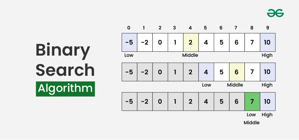
To see this in action, let's watch a short video that walks through the logic and, importantly, highlights a common and subtle bug in many binary search implementations.

Implementing Binary Search

Now that we have the core idea, let's translate it into code. Binary search can be implemented in two main ways: iteratively (using a loop) or recursively. The iterative approach is generally preferred in production code because it avoids the overhead of function calls and uses constant extra space.

The following article provides well-explained code for both approaches.

Common Pitfalls

Even though the concept is simple, implementing binary search correctly can be tricky. Here are some of the most common mistakes, which the article you just reviewed also mentions in its "Common Mistakes and Pitfalls" section:

• Off-by-One Errors: Incorrectly updating the left and right boundaries (e.g., right = mid instead of right = mid - 1) can lead to infinite loops or incorrect results. Always trace your logic with a small example to be sure.
• Integer Overflow: As the video highlighted, using mid = (left + right) / 2 can cause an overflow if left and right are very large positive numbers. The safer mid = left + (right - left) / 2 avoids this.
• Incorrect Loop Condition: The loop should continue as long as left <= right. If you use left < right, the algorithm will fail to check the final element when the search space shrinks to a single item.

Analyzing the Complexity

The real power of binary search lies in its efficiency. Let's analyze its time and space complexity.

Time Complexity: The Power of Logarithms

As you've seen, binary search halves the search space with every comparison. This "halving" is the key to its logarithmic time complexity.

To build a strong intuition for this, let's watch a short clip that directly connects the halving process to logarithms.

Now, let's formalize this with a mathematical derivation. For an array of size $n$, the search space is reduced as follows:

• After 1 comparison: $n/2$ elements remain.
• After 2 comparisons: $n/4$ elements remain.
• After $k$ comparisons: $n/2^k$ elements remain.

The search terminates in the worst case when the search space is reduced to 1 element. So, we set the remaining size to 1 and solve for $k$, the number of comparisons:

This shows that the number of comparisons is logarithmic with respect to the input size.

For a more rigorous look, including an analysis using recurrence relations (which you may find familiar from your engineering studies), the following resource is excellent.

To summarize the time complexity:

• Best Case: $O(1)$. The target is the middle element on the first check.
• Average Case: $O(\log n)$. On average, the target is found after a logarithmic number of steps.
• Worst Case: $O(\log n)$. The target is found at the last possible step, or it is not in the array at all.

Space Complexity

The space complexity depends on the implementation:

• Iterative Implementation: $O(1)$. We only use a few variables (left, right, mid) to keep track of the search. The amount of extra space is constant and does not grow with the input size $n$.
• Recursive Implementation: $O(\log n)$. Each recursive call adds a new frame to the call stack. In the worst case, the recursion depth is $\log n$, so the space used by the call stack is proportional to $\log n$.

Conclusion

In this lesson, we've taken a deep dive into binary search, a cornerstone algorithm for any developer. Its efficiency makes it indispensable when working with large, sorted datasets.

Key Takeaways:

• Binary search operates on sorted arrays using a divide and conquer strategy.
• It has a logarithmic time complexity, $O(\log n)$, because it halves the search space in each step.
• The iterative implementation is generally preferred due to its constant space complexity, $O(1)$.
• Correct implementation requires careful handling of boundary conditions and using an overflow-safe method to calculate the middle index.

Preview of the Next Lesson:

You now understand several sorting algorithms (Merge Sort, Quicksort, Counting Sort) and a powerful searching algorithm (Binary Search). The next logical step is to know when to use which. In our next lesson, we will focus on the final outcome of this module: "Select an appropriate sorting or searching strategy based on problem constraints." We'll analyze trade-offs and develop a mental framework for making these critical design decisions.