Pruning for Backtracking Optimization

1. The Core Idea: Pruning the State-Space Tree

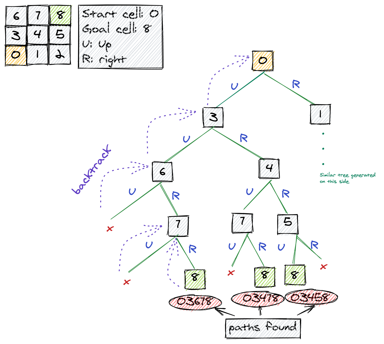
As we've discussed, backtracking can be visualized as a depth-first search on a state-space tree, where each node is a partial solution. A naive algorithm might explore every possible branch until it hits a leaf, only then realizing the path was invalid. This is computationally expensive.

Pruning is the process of identifying and "cutting off" branches of this tree as early as possible, as soon as we can determine they cannot possibly lead to a valid solution. The function or logic that makes this decision is often called a bounding function.

To see a simple illustration of this, let's watch a brief segment from a video by Abdul Bari.

This simple example perfectly illustrates the goal. By applying a bounding function, we saved the work of exploring invalid branches. In more complex problems, this "saved work" can mean the difference between an algorithm that finishes in seconds and one that would run for years.

As noted in the lecture notes from Stony Brook University, efficiency in backtracking comes almost entirely from this concept.

2. A Pattern for Pruning: construct_candidates

So, how do we implement pruning effectively? While our isSafe() checks in previous lessons worked, a more structured and often more efficient approach is to separate the generation of valid moves from the recursive exploration.

A common pattern is to use a helper function, often named construct_candidates, whose job is to build a list of all valid next moves from the current state. The main recursive function then simply iterates over this pre-vetted list. This moves the pruning logic into its own dedicated function.

The pseudocode for this pattern looks like this:

backtrack(partial_solution, k):
  if partial_solution is a complete solution:
    process_solution(partial_solution)
    return

  // Pruning happens here:
  candidates = construct_candidates(partial_solution, k)

  // Exploration happens here:
  for each candidate c in candidates:
    add c to partial_solution
    backtrack(partial_solution, k+1)
    remove c from partial_solution // Backtrack

This pattern is cleaner because the main backtrack function only orchestrates the search, while construct_candidates handles the problem-specific constraints and pruning.

Let's look at a concrete example within the N-Queens problem from the same lecture notes.

The function you just reviewed prunes the search space by ensuring the recursive backtrack function is never even called for an invalid queen placement. The key question now becomes: how can we make those legal_move checks as fast as possible?

3. Case Study: High-Efficiency Pruning in N-Queens

The construct_candidates function from the PDF uses a loop to check for threats, which runs in $O(k)$ time for the $k$-th queen. For large $N$, this can be slow. Can we do better?

Yes, by using data structures that allow us to check for threats in constant, $O(1)$ time. This is a common theme in algorithm optimization that leverages your software engineering expertise. The key is to find a way to represent the board's constraints mathematically.

For N-Queens, the constraints are:

1. No two queens in the same column.
2. No two queens in the same row (handled by placing one queen per row).
3. No two queens on the same diagonal.

The column check is easy: we can use a set to store occupied column indices. The diagonal check is trickier, but there's a clever mathematical property we can exploit.

Let's watch a video that explains this property and then uses it to build a highly efficient N-Queens solver.

This implementation is a prime example of effective pruning. Instead of a loop, a few set lookups instantly determine if a branch of the search tree should be pruned. The "choose" step involves adding to the sets, and the "unchoose" step involves removing from them. This is a far more performant approach than the one we saw in the C pseudocode.

4. Other Pruning Strategies

The techniques we've focused on—using bounding functions and efficient data structures—are fundamental. But there are other, often problem-specific, strategies to be aware of.

• Constraint Propagation: As we previewed in the Sudoku lesson, sometimes placing a value in one spot logically determines the value in another. Solving for these determined values without making a "choice" and recursing is a powerful form of pruning because it reduces the depth and breadth of the search tree. The Sudoku paper (LINK) details this in its reduce(grid) procedure, which fills in all 'fixed' cells before the next recursive step.

• Symmetry Exploitation: In many problems, some solutions are just symmetric versions of others (e.g., rotations or reflections). For N-Queens, if you find one solution, you can often generate up to 7 others for free by reflecting and rotating the board. By adding logic to avoid searching for these symmetric solutions, you can prune massive sections of the search space. Skiena's lecture notes (LINK) mention this in the section "Exploiting Symmetry."

• Heuristics (Ordering of Choices): As we also saw with Sudoku's "Minimum Remaining Values" heuristic, the order in which you explore choices matters. Trying to place a value in the most constrained cell first often leads to failures faster, which prunes the tree higher up, yielding an exponential speedup.

Conclusion

This lesson concludes our deep dive into backtracking. We've seen that while the basic recursive structure is simple, its practical application relies heavily on intelligent and aggressive pruning of the state-space tree.

Key Takeaways:

• Pruning is the process of eliminating branches from the state-space tree that cannot lead to a solution. It is the single most important factor for backtracking efficiency.
• A bounding function is the logical test used to decide whether to prune a branch.
• The construct_candidates pattern is a clean way to implement pruning by separating the logic for generating valid moves from the recursive search itself.
• Using appropriate data structures (like sets for the N-Queens problem) can make constraint checking—and thus pruning—dramatically more efficient, often reducing it to $O(1)$ time.
• Advanced techniques like constraint propagation and exploiting symmetry can offer further, often massive, reductions in the search space.

Preview of the Next Module:

We have now covered several major algorithmic paradigms: sorting, searching, divide and conquer, greedy algorithms, and backtracking. We are now ready to tackle problems on a new and powerful data structure: graphs. In the next module, Graph Traversal Techniques, we will begin by learning the two primary ways to represent a graph in memory: the adjacency matrix and the adjacency list. Understanding their trade-offs is the foundation for all the graph algorithms that will follow.